Simulating Life: The Final Sanctuary of Artificial Intelligence

写作说明 / Note

本文由 AI（Trae Agent） 检索、整理并撰写，尚未经过人工逐条校对。文中所有数字都来自随文附带的 Python 脚本的真实运行结果（experiments/01_language.py 至 06_conceptual.py），在 CPU 上即可重跑；图表由这些脚本直接生成，未做手工修改。所有”虚拟细胞”都是玩具模型，不构成任何关于真实细胞、真实物种或临床应用的结论。文献条目给出 DOI 或机构链接；无法核实的 DOI 一律不写。

This article was researched and written by an AI system (Trae Agent) and has not been proofread line by line by a human. Every number comes from an actual run of the Python scripts shipped with the post (experiments/01_language.py … 06_conceptual.py), which run on a CPU; all figures are produced by those scripts and are not retouched. The “virtual cell” here is a toy model and says nothing about real cells, organisms or clinical use. References carry DOIs or institutional links; no DOI is invented.

生成本文所用的提示词（压缩后） / Prompt used to generate this article (condensed)

写一篇中英双语长文《生命模拟：人工智能的最后圣殿》。用一个思想实验开篇：能生成任何句子、任何图像、整个物理世界的计算机，能否”创造”生命？按”识别—生成—预测—模拟—干预—生命模拟”梳理 AI 的范式扩展。用 Python 做四组可复现实验：人工语法上的小型语言模型、Fashion-MNIST 上的 VAE、阻尼受迫摆上的黑箱与结构化模型对比、以及一个十基因虚拟细胞及其扰动预测。必须包含：训练曲线、泛化与分布外结果、干预预测、一个能挑战中心论点的负面实验；讨论 AlphaFold、AlphaGenome、Arc Institute 的 STATE 与 Virtual Cell Challenge；区分”模拟”“理解”“创造”；所有数字来自真实运行，图表由代码生成。

A long bilingual essay, Simulating Life: The Final Sanctuary of Artificial Intelligence, opening with a thought experiment: a machine that can generate any sentence, any image and an entire physical world — can it create life? Trace the widening of AI’s remit: recognition, generation, prediction, simulation, intervention, living systems. Four reproducible Python experiments: a tiny language model on an artificial grammar, a VAE on Fashion-MNIST, black-box versus structured models of a driven pendulum, and a ten-gene virtual cell with perturbation prediction. Include training curves, out-of-distribution results, intervention tests and one negative result that challenges the thesis; discuss AlphaFold, AlphaGenome, Arc’s STATE and the Virtual Cell Challenge; distinguish simulating, understanding and creating. Every number must come from an actual run, and every figure from code.

1. 三个房间，一个问题 / Three rooms, one question

假设我们有三个房间。第一个房间里是一台能写出任何合语法句子的机器；第二个房间里是一台能画出任何图像的机器；第三个房间里是一台能模拟整个物理世界的机器——给定初始条件与力，它推演每一个粒子的轨迹。现在把一个问题放进这三个房间：它们之中，有哪一台能创造出一个会生长、会适应、会复制自己、并在长期演化中产生新行为的系统？

Imagine three rooms. In the first, a machine that can write any grammatical sentence; in the second, one that can draw any image; in the third, one that can simulate the entire physical world — give it initial conditions and forces, and it follows every particle. Now put one question into all three rooms: which of them can create a system that grows, adapts, copies itself, and produces new behaviour over long timescales?

这个问题需要先做一个限定。这里的”创造”指的是在计算世界里构造一个可运行的系统，而不是声称在实验室里合成了生命。本文讨论的是模拟（simulation），不是合成（synthesis）。这个限定看似退让，实际上把问题变得更难，因为它剥夺了所有含糊其辞的余地：如果一个系统在计算机里既不能自我维持，也不能对环境作出可检验的响应，那它就不是生命模拟，只是生命动画。

The question needs one restriction. “Create” here means build a runnable system inside a computer, not claim that life has been synthesised in a laboratory. This article is about simulation, not synthesis. The restriction looks like a concession but makes the problem harder, because it removes every escape route: if a system cannot maintain itself and cannot respond to its environment in a testable way, it is not a life simulation, only an animation of life.

1.1 从识别到模拟，问题在变宽 / From recognition to simulation, the question widens

过去十五年，AI 的进展可以被读成一条问题变宽的序列。最早的问题是”这张图里有没有猫”，答案是一个标签；然后是”给我一张像猫的图”，答案是一个样本；再然后是”下一帧会是什么”，答案是未来；再往后是”如果我把这个关节推一下，整条手臂会怎么动”，答案是干预之后的世界。每一步都不是前一步的替代品，而是把”模型必须回答什么”这件事向前推了一格。

Fifteen years of AI progress can be read as a sequence of widening questions. First: “is there a cat in this image” — the answer is a label. Then: “give me an image that looks like a cat” — the answer is a sample. Then: “what comes next” — the answer is a future. Then: “if I push this joint, how does the arm move” — the answer is a world after an intervention. Each step replaces nothing; it moves the question one notch outward.

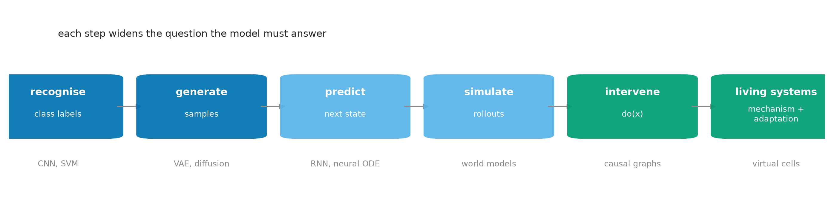
图 1　AI 建模范式的六个阶段。每个阶段不是替代前一个，而是把模型必须回答的问题向前推一格：从”是什么”到”像什么”，到”接下来是什么”，到”如果这样做会怎样”，最后到”这个系统能不能自己维持下去”。 | Figure 1. Six stages in AI modelling. Each stage does not replace the previous one; it pushes the question one notch outward: from “what is it” to “what does it look like”, to “what comes next”, to “what happens if I do this”, and finally to “can the system keep itself alive”. — **图 1**　AI 建模范式的六个阶段。每个阶段不是替代前一个，而是把模型必须回答的问题向前推一格：从”是什么”到”像什么”，到”接下来是什么”，到”如果这样做会怎样”，最后到”这个系统能不能自己维持下去”。 | **Figure 1.** Six stages in AI modelling. Each stage does not replace the previous one; it pushes the question one notch outward: from “what is it” to “what does it look like”, to “what comes next”, to “what happens if I do this”, and finally to “can the system keep itself alive”.

用表格列出这条线上最常被引用的技术，会看得更清楚。它们之间不是”新旧替代”，而是各自补上了一块此前缺失的能力。

A table of the techniques usually cited along this line makes the pattern clearer. They do not supersede one another; each supplies a capability that was missing before.

阶段 / Stage	代表方法 / Representative methods	它新增了什么 / What it adds
识别 / recognise	CNN、ViT	把高维输入压成一个语义标签 / a high-dimensional input becomes a label
生成 / generate	VAE、GAN、diffusion	学会整个数据分布，而不只是判别边界 / the whole distribution, not just a boundary
预测 / predict	RNN、Transformer、neural ODE	状态随时间的转移 / state transitions in time
模拟 / simulate	world models、neural operators	多步 rollout 与守恒量 / multi-step rollouts and invariants
干预 / intervene	因果图、do-calculus、扰动数据	“做”与”看”的差别 / the difference between doing and seeing
生命 / living systems	多尺度机理模型、虚拟细胞	自我维持、适应与历史性 / self-maintenance, adaptation, history

English: the same table, one row per stage; the third column is the capability the stage added.

1.2 四个”世界”的形状不同 / The four worlds have different shapes

把语言、图像、物理与生命并置时，最常见的错误是以为它们只是”难度不同”的同一个问题。它们的状态空间形状根本不同：语言是离散符号上的链，图像是连续空间里的低维流形，物理是带守恒量的轨道，生命则是一个有多个吸引子的景观，而且景观本身会随历史改变。

When language, images, physics and life are placed side by side, the usual mistake is to assume they are the same problem at different difficulty levels. Their state spaces have different shapes: language is a chain over discrete symbols, images a low-dimensional manifold in a continuous space, physics an orbit constrained by conservation laws, and life a landscape with several attractors — a landscape that history itself can reshape.

图 2　四种”世界”的状态空间示意。语言是离散链；图像分布在光滑流形附近；物理轨道被守恒量约束；生命系统有多个稳定状态，而扰动可能把系统从一个吸引子推到另一个。这张图是示意，不是数据。 | Figure 2. Schematic state spaces for the four worlds. Language is a discrete chain; images lie near a smooth manifold; physical orbits are constrained by conservation laws; living systems have several stable states, and a perturbation can push the system from one attractor to another. This figure is a diagram, not data. — **图 2**　四种”世界”的状态空间示意。语言是离散链；图像分布在光滑流形附近；物理轨道被守恒量约束；生命系统有多个稳定状态，而扰动可能把系统从一个吸引子推到另一个。这张图是示意，不是数据。 | **Figure 2.** Schematic state spaces for the four worlds. Language is a discrete chain; images lie near a smooth manifold; physical orbits are constrained by conservation laws; living systems have several stable states, and a perturbation can push the system from one attractor to another. This figure is a diagram, not data.

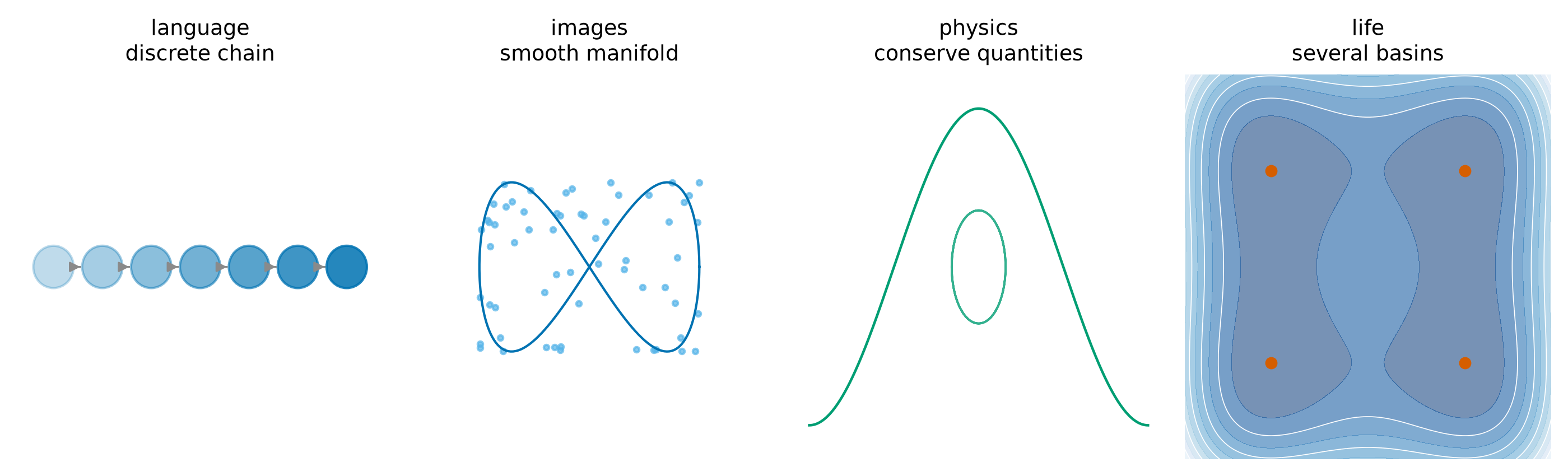
这张图没有数据，它是后面所有实验的”提问方式”：如果我们想知道某一类模型是否真的理解了它所在的世界，就要问它对这个形状做了什么——是记住了样本，还是学到了流形；是拟合了轨迹，还是学到了守恒量；是预测了下一次观测，还是能预测一次从未做过的干预。

This figure contains no data; it sets the way the rest of the article asks questions. To know whether a model has understood its world, ask what it did with that shape: did it memorise samples or learn the manifold; fit trajectories or learn the invariants; predict the next observation or predict an intervention that has never been performed.

2. 语言：符号的世界 / Language: the world of symbols

第一个实验刻意做得很小，因为小才看得清。我们不去训练一个大语言模型，而是造一门语言：它有明确的语法，因此”这句话合不合法”可以独立判定；它还有一条长距离依赖，因此”模型有没有学到结构”可以被单独测量。

The first experiment is deliberately small, because small is legible. Instead of training a large language model, we invent a language: it has an explicit grammar, so “is this sentence grammatical” can be decided independently, and it has a long-distance dependency, so “did the model learn structure” can be measured on its own.

这门语言里有两个约束。第一，冠词与名词必须数一致（a fox 可以，a foxes 不行）。第二，主句动词必须与主语名词数一致，即使中间隔着一整个关系从句：the cat that the dogs chase runs——runs 呼应的是 cat，不是离它更近的 dogs。第二条是关键：一个只统计相邻词对的模型会在这里出错。

The language has two constraints. First, determiner and noun must agree in number (a fox is fine, a foxes is not). Second, the main verb must agree with the subject noun even when an entire relative clause sits between them: the cat that the dogs chase runs — runs agrees with cat, not with the nearer dogs. The second constraint is the point: a model that only counts adjacent pairs will fail here.

我们生成了 18,000 条句长为 3–14 个词的句子（平均 8.5 个词），词表只有 20 个符号。模型是一个单层 GRU 加一个线性输出层，训练目标只有一件事：给定前文，预测下一个词。我们训练了两个尺寸（隐藏层 32 与 96），因为”数据里有结构”与”这个模型能用上结构”是两个不同的问题。

We generated 18,000 sentences of 3–14 words (mean 8.5), over a vocabulary of only 20 symbols. The model is a single-layer GRU with a linear readout, trained on one objective only: given the prefix, predict the next token. Two sizes were trained (hidden width 32 and 96), because “the data has structure” and “this model can use it” are different questions.

图 3　(a) 两个尺寸语言模型的验证损失：都在第 2–3 轮后进入平台，说明这门语言本身的熵很高，局部规律很快就学完了。 (b) 在训练长度内（浅色区）与超出训练长度的句子上，每 token 的比特数——压缩一个未见句子所需的成本。 | Figure 3. (a) Validation loss of the two language models; both plateau after two or three epochs, which says the corpus itself is high-entropy and the local regularities are learned quickly. (b) Bits per token on held-out sentences inside (shaded) and beyond the training lengths — the cost of compressing an unseen sentence. — **图 3**　(a) 两个尺寸语言模型的验证损失：都在第 2–3 轮后进入平台，说明这门语言本身的熵很高，局部规律很快就学完了。 (b) 在训练长度内（浅色区）与超出训练长度的句子上，每 token 的比特数——压缩一个未见句子所需的成本。 | **Figure 3.** (a) Validation loss of the two language models; both plateau after two or three epochs, which says the corpus itself is high-entropy and the local regularities are learned quickly. (b) Bits per token on held-out sentences inside (shaded) and beyond the training lengths — the cost of compressing an unseen sentence.

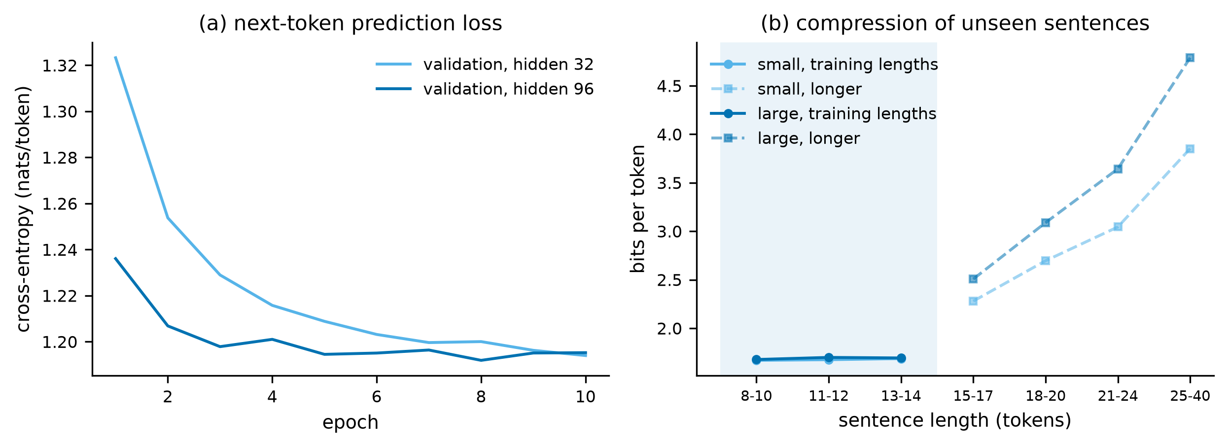
两个模型都收敛到大约 1.20 nats/token，即每词约 1.72 比特。这个数字要小心解读：它不是说模型”学得不好”，而是这门语言本身在每个位置上都有相当大的不确定性——冠词有 2 种、名词有 8 种、动词形式有 6 种，很多选择在语法上同时合法。低损失不等于理解，高损失也不等于没学到。

Both models converge to about 1.20 nats per token, that is 1.72 bits per word. The number needs care: it does not say the models learned badly, it says the language itself carries a lot of uncertainty at each position — two determiners, eight nouns, six verb forms, and many choices are simultaneously grammatical. Low loss is not understanding, and high loss is not failure to learn.

2.1 它会造句，而且句法正确 / It generates sentences, and they parse

自由生成 400 条句子，用独立的递归下降解析器判定合法性（这个解析器刻意不复用生成器的任何代码，否则测的就是自己）。小模型 98.8% 的句子合法，大模型 99.8%。以下是两条真实生成的句子，均来自 400 条样本：

400 sentences were sampled freely and checked with an independent recursive-descent parser (deliberately sharing no code with the generator, otherwise the test would grade itself). 98.8% of the small model’s sentences parse, and 99.8% of the large model’s. Two actual samples from the 400:

a fox sees the birds that the birds like

the foxes that the dog likes chase

第一句里，主句动词 likes 与主语 cat 一致，而它们之间隔着一个关系从句 that the foxes that the foxes chase like。模型从来没有被教过”主谓一致”这条规则，它只是被要求预测下一个词。规则可以从分布中学到，这是这个实验最干净的一半结论。

In the first sentence the main verb likes agrees with cat, across the relative clause that the foxes that the foxes chase like. The model was never taught the rule of subject–verb agreement; it was only asked to predict the next token. Rules can be learned from a distribution — that is the clean half of this experiment’s conclusion.

2.2 学到的规则有多结实？ / How robust is the learned rule?

“会造句”还不够。真正的问题是：这条长距离依赖在距离变大时还成立吗？我们构造了一批前缀，把动词之前、主语名词之后的词数从 2 拉到 30，然后比较模型给正确动词形式与错误形式的概率。

Generating sentences is not enough. The real question is whether the dependency survives as the distance grows. We built prefixes with 2 to 30 tokens between the subject noun and the verb, then compared the probability the model assigns to the correct versus the incorrect verb form.

图 4　(a) 自由生成句子的长度分布。两个模型几乎不生成超过训练长度（虚线 14 个词）的句子，尽管语法允许无限长。 (b) 长距离一致性：纵轴是”正确形式的对数概率减去错误形式的对数概率”，越大表示越有把握。距离在 10 个词以内时两个模型都很稳，到 15–30 个词时大模型只剩 0.42 nats 的优势，小模型只剩 0.18。 | Figure 4. (a) Length distribution of freely generated sentences; both models stay inside the training range (dashed line at 14 words) although the grammar allows unbounded length. (b) Long-distance agreement: the vertical axis is log p(correct) − log p(wrong), so larger is more confident. Both models are stable up to about ten intervening tokens; at 15–30 the large model retains a margin of 0.42 nats and the small one only 0.18. — **图 4**　(a) 自由生成句子的长度分布。两个模型几乎不生成超过训练长度（虚线 14 个词）的句子，尽管语法允许无限长。 (b) 长距离一致性：纵轴是”正确形式的对数概率减去错误形式的对数概率”，越大表示越有把握。距离在 10 个词以内时两个模型都很稳，到 15–30 个词时大模型只剩 0.42 nats 的优势，小模型只剩 0.18。 | **Figure 4.** (a) Length distribution of freely generated sentences; both models stay inside the training range (dashed line at 14 words) although the grammar allows unbounded length. (b) Long-distance agreement: the vertical axis is log p(correct) − log p(wrong), so larger is more confident. Both models are stable up to about ten intervening tokens; at 15–30 the large model retains a margin of 0.42 nats and the small one only 0.18.

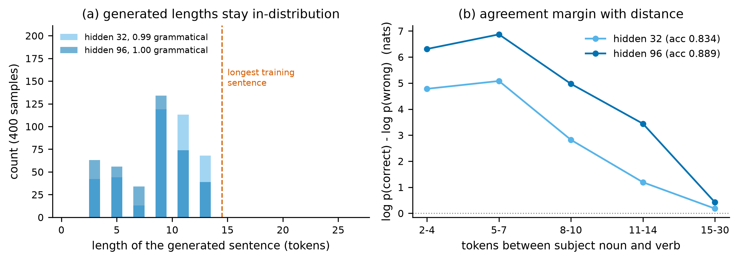
这里出现了第一个”能力的边界”。在 2–9 个词的距离上，两个模型的判断都是 100% 正确；到 11–14 个词时正确率降到 92.9%；到 15–30 个词时只剩 51.4%。也就是说：模型学到的是”在这门语言的典型长度上成立”的规则，而不是”在语法允许的任何长度上都成立”的规则。 训练数据里没有长句子，模型也就不生成长句子（图 4a），这正是”分布内很像、分布外很脆”的标准形态。

Here is the first boundary. At distances of 2–9 tokens both models are right 100% of the time; at 11–14 tokens the large model falls to 92.9%; at 15–30 it is 51.4%. In other words: the model learned a rule that holds at the lengths typical of this language, not a rule that holds at every length the grammar permits. The training data contain no long sentences, and the model generates none (Figure 4a) — the standard shape of “faithful inside the distribution, brittle outside it”.

图 3(b) 给出了同一件事的另一个读数：在训练长度内，压缩一个未见句子只要 1.68 比特/词；到了 18–20 个词变成，25–40 个词变成 2.51。这不是”模型变笨了”，而是它被要求处理一个它从未见过的长度。

Figure 3b gives another reading of the same fact: inside the training lengths an unseen sentence costs 1.68 bits per token; at 18–20 words it costs , and at 25–40 words 2.51. The model did not become stupid; it was asked to handle a length it had never seen.

2.3 为什么”下一词预测”不等于理解世界 / Why next-token prediction is not world understanding

结论需要说得比”语言模型很强”更精确。这个模型展示了三件事：语法可以从分布中学到；规则的使用会随着偏离训练分布而退化；以及——最重要的一件——整个实验里没有任何”世界”。句子不指涉任何对象，没有真假，没有因果。模型学到的是符号之间的转移概率，而”猫”这个词在这里没有任何四条腿。

The conclusion has to be more precise than “language models are strong”. This model shows three things: grammar is learnable from a distribution; the use of a rule degrades as you leave that distribution; and — most importantly — there is no world anywhere in this experiment. The sentences denote nothing, are neither true nor false, and have no causal content. What the model learned is a transition probability between symbols, and the word “cat” has no legs here.

这一点必须与”语言模型不懂物理”的常见论调区分开。语言模型当然可以在文本里学到大量关于世界的相关结构——“玻璃杯掉到地上会碎”在语料里出现得足够多。但相关结构可以支撑预测，却不足以支撑干预：如果我从没见过的角度推一个杯子，它会不会碎？这个问题在语料里没有答案，因为没有人写过。第 4 节会把这个区别做成实验。

This must be distinguished from the loose claim that “language models don’t understand physics”. A language model can certainly learn a great deal of correlational structure about the world from text — “a glass dropped on the floor breaks” appears often enough. Correlational structure supports prediction but not intervention: if I push the glass from an angle nobody has described, will it break? The corpus contains no answer, because nobody wrote one. Section 4 turns this distinction into an experiment.

3. 图像：感知的世界 / Images: the world of perception

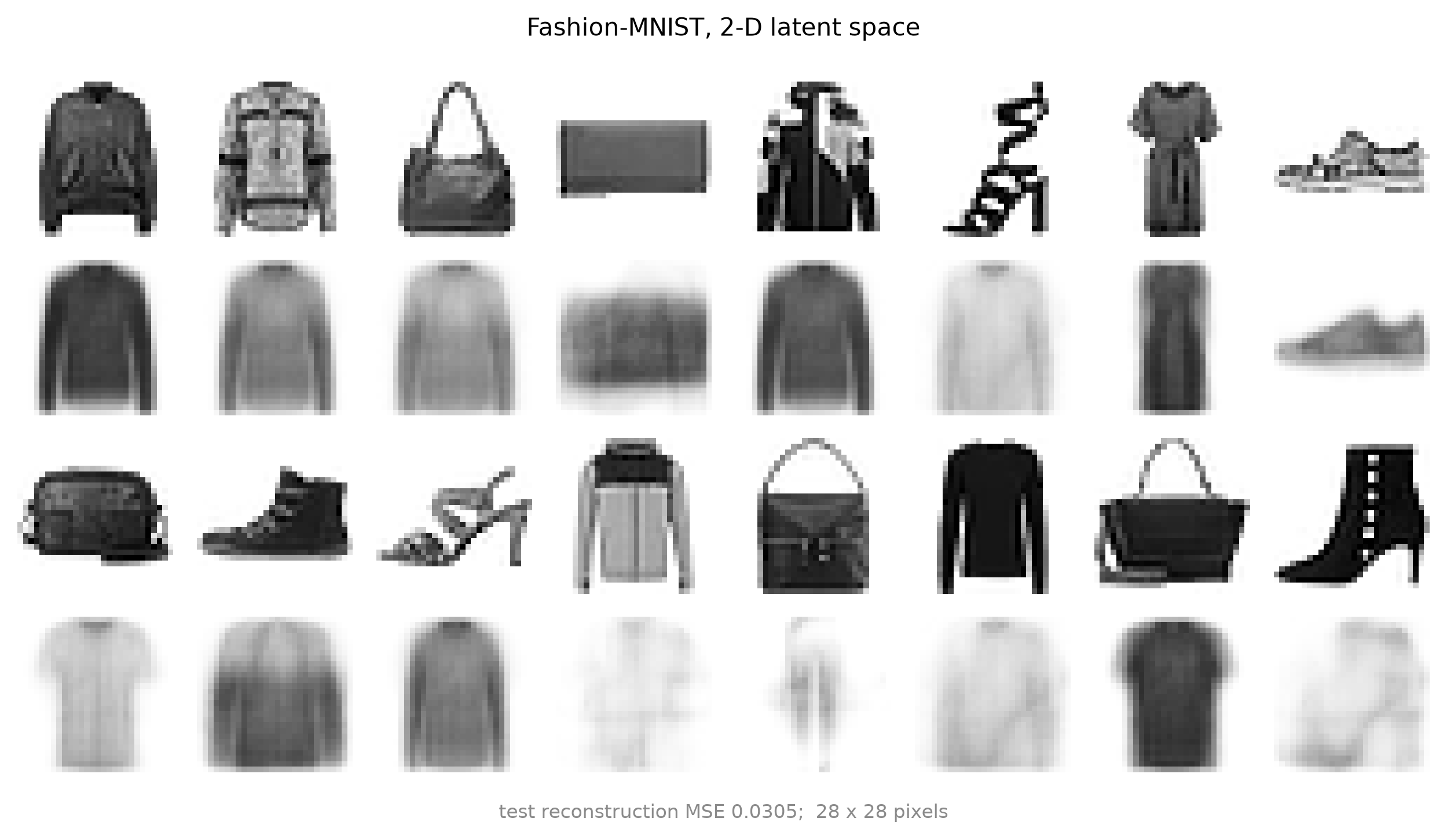
第二个实验换成连续空间。我们训练一个变分自编码器（VAE），把 28×28 的 Fashion-MNIST 图像压进一个二维潜在空间。二维是刻意的妥协：它牺牲了重建质量，换来一个可以直接看、直接量的几何结构。训练集 20,000 张，15 轮，最后的验证 ELBO 约为 270 nats/图。

The second experiment moves to a continuous space. A variational autoencoder compresses 28×28 Fashion-MNIST images into a two-dimensional latent space. Two dimensions are a deliberate compromise: reconstruction suffers, but the geometry becomes something you can look at and measure directly. 20,000 training images, 15 epochs, final validation ELBO about 270 nats per image.

图 5　重建与采样。第 1、3 行是输入，第 2 行是模型用潜在均值重建的图像，第 4 行是从先验采样的图像。测试集重建 MSE 为 0.0305。重建明显模糊——这是二维瓶颈的直接代价，不是训练失败。 | Figure 5. Reconstruction and sampling. Rows 1 and 3 are inputs, row 2 reconstructions from the latent mean, row 4 samples from the prior. Test reconstruction MSE is 0.0305. The blur is the direct price of a two-dimensional bottleneck, not a training failure. — **图 5**　重建与采样。第 1、3 行是输入，第 2 行是模型用潜在均值重建的图像，第 4 行是从先验采样的图像。测试集重建 MSE 为 0.0305。重建明显模糊——这是二维瓶颈的直接代价，不是训练失败。 | **Figure 5.** Reconstruction and sampling. Rows 1 and 3 are inputs, row 2 reconstructions from the latent mean, row 4 samples from the prior. Test reconstruction MSE is 0.0305. The blur is the direct price of a two-dimensional bottleneck, not a training failure.

图 6　潜在空间与插值。(a) 测试集在二维潜在空间中的位置，颜色是真实类别；类别不是完全分离的，但显然不是随机的。(b) 两个凉鞋的潜在编码之间做线性插值再解码，中间状态是平滑的过渡，而不是突变。 | Figure 6. Latent space and interpolation. (a) Test images in the two-dimensional latent space, coloured by true class; the classes are not perfectly separated but are clearly not random. (b) Linear interpolation between the latent codes of two sandals, decoded; intermediate states are smooth transitions rather than jumps. — **图 6**　潜在空间与插值。(a) 测试集在二维潜在空间中的位置，颜色是真实类别；类别不是完全分离的，但显然不是随机的。(b) 两个凉鞋的潜在编码之间做线性插值再解码，中间状态是平滑的过渡，而不是突变。 | **Figure 6.** Latent space and interpolation. (a) Test images in the two-dimensional latent space, coloured by true class; the classes are not perfectly separated but are clearly not random. (b) Linear interpolation between the latent codes of two sandals, decoded; intermediate states are smooth transitions rather than jumps.

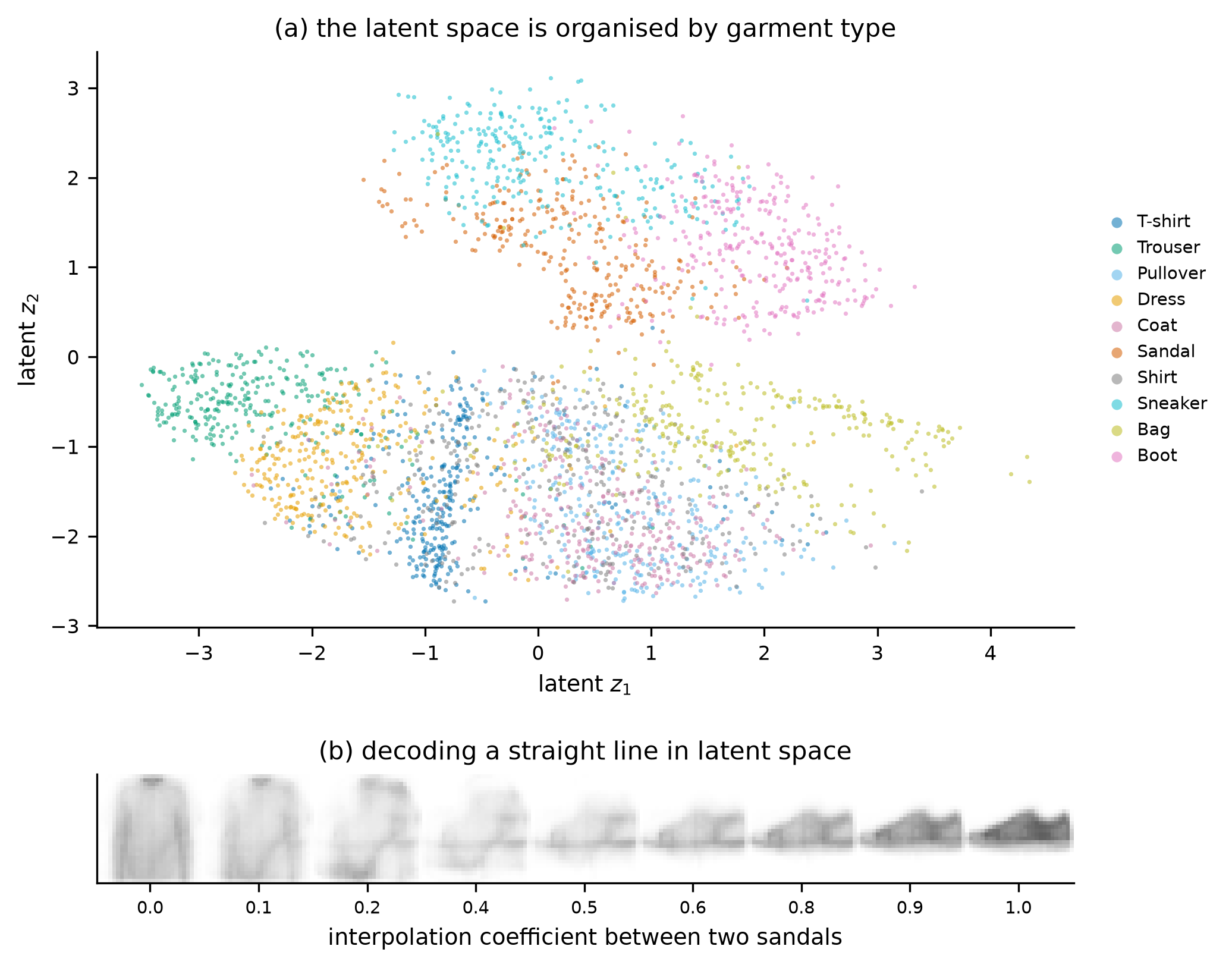
这张潜在空间图值得多看一会儿。它说明模型学到了连续的、按语义组织的坐标：位置相近的图像在视觉上也相近，插值路径上的每一帧都是一个”像衣服的东西”。这已经是真正的结构，不是记忆：模型在训练中从未见过插值路径上的那些点。

The latent figure deserves a pause. It shows that the model learned continuous, semantically organised coordinates: nearby codes correspond to visually similar images, and every frame along the interpolation path looks like a garment. That is genuine structure, not memorisation: the model never saw those intermediate points during training.

但同一张图也标出了这个结构的边界。潜在空间只保证”在数据流形上平滑”，不保证”在流形外有意义”。我们可以用四个分布外的探针来量这件事：

But the same figure marks the boundary of that structure. A latent space guarantees smoothness on the data manifold, not meaning off it. Four out-of-distribution probes measure the difference:

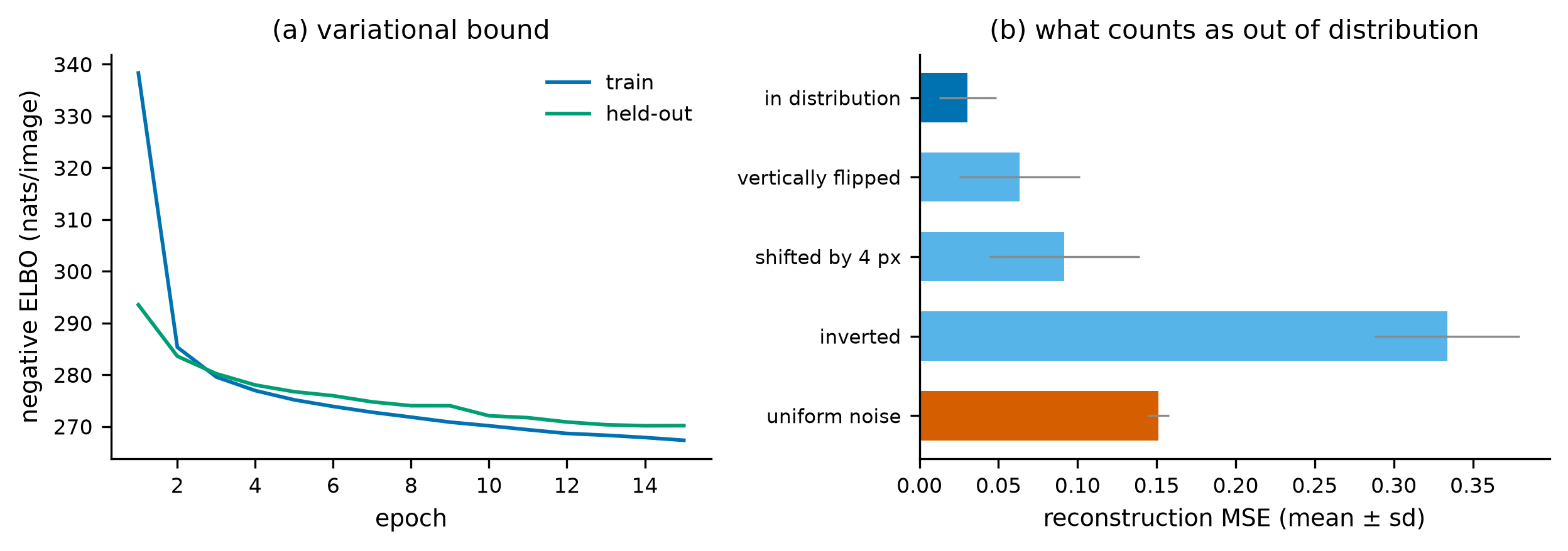
图 7　分布外探针。纵轴是五类输入的重建 MSE（均值 ± 标准差）：原图、上下翻转、平移 4 像素、反色、均匀噪声。模型对”翻转”和”平移”的重建误差只比原图高一点，对”反色”则高出约十倍。 | Figure 7. Out-of-distribution probes. Bars show reconstruction MSE (mean ± sd) for the original images, vertical flip, a four-pixel shift, inversion, and uniform noise. Flips and shifts cost little; inversion costs about ten times more. — **图 7**　分布外探针。纵轴是五类输入的重建 MSE（均值 ± 标准差）：原图、上下翻转、平移 4 像素、反色、均匀噪声。模型对”翻转”和”平移”的重建误差只比原图高一点，对”反色”则高出约十倍。 | **Figure 7.** Out-of-distribution probes. Bars show reconstruction MSE (mean ± sd) for the original images, vertical flip, a four-pixel shift, inversion, and uniform noise. Flips and shifts cost little; inversion costs about ten times more.

数字很有意思。原图的重建 MSE 是 0.0305；上下翻转是 0.0632，平移 4 像素是 0.0916——模型对几何变换相当宽容。但反色是 0.3337，均匀噪声是 0.1512。“看起来仍然是一张图”与”在模型的坐标系里有意义”不是一回事。

The numbers are informative. Original reconstruction MSE is 0.0305; a vertical flip costs 0.0632, a four-pixel shift 0.0916 — the model is tolerant of geometric transforms. Inversion costs 0.3337 and uniform noise 0.1512. “Still looks like an image” and “is meaningful in the model’s coordinate system” are different properties.

这里要防止一个常见的过度解读。生成模型能画出逼真的图像，不等于它拥有对象恒常性、三维几何或因果推理。我们的 VAE 能重建一只鞋，但它不知道鞋有两只、不知道鞋会掉下去、不知道把鞋翻过来里面是空的。图 7 的翻转实验甚至说明：它对”上下”这个概念几乎没有表示，只是把翻转后的图像当作另一个样本。

One common over-reading must be blocked. A generative model producing realistic images does not imply object permanence, three-dimensional geometry or causal reasoning. Our VAE can reconstruct a shoe, but it does not know that shoes come in pairs, that they fall, or that turning one over reveals an empty inside. The flip probe in Figure 7 suggests it barely represents “up”: a flipped image is simply another sample.

视频生成把这一点推得更远，也更危险。视频模型能生成”物体被遮挡后重新出现”的画面，看起来像对象恒常性；但这同样可以由像素的时间相关性解释，不需要一个关于”物体持续存在”的内部变量。判断标准只有一个：模型能否在干预之下仍然正确。 遮挡是观测，移走是干预。这两者在视频数据里的分布不同，而在真实世界里后果不同。

Video generation pushes this further, and makes it more seductive. A video model can produce an object that reappears after occlusion, which looks like object permanence; but temporal pixel correlation explains that too, without any internal variable for “the object persists”. The test is whether the model stays correct under intervention. Occlusion is an observation; removal is an intervention. They have different distributions in video data and different consequences in the world.

4. 非生命：物理规律的世界 / Non-life: the world of physical law

在跳到生命之前，必须经过物理。原因不是物理”更简单”，而是物理提供了一个干净的对照：在这个世界里，我们同时拥有数据和一个已知的生成机制。 于是可以问一个在生物学里很难问的问题——当数据和机制同时存在时，模型到底学到了哪一个？

Physics is the necessary stop before life. Not because it is “easier”, but because it provides a clean control: here we have both the data and a known generating mechanism. That permits a question that is hard to ask in biology — when data and mechanism are both available, which one does the model learn?

4.1 系统与两种模型 / The system and two models

我们用一个阻尼受迫摆：

We use a damped, periodically driven pendulum:

\[ \ddot\theta = -\gamma\,\dot\theta - \sin\theta + A\cos(\omega t) \]

状态是 $(\theta,\dot\theta)$，控制参数是阻尼 $\gamma$ 与驱动幅度 $A$。数据由四阶 Runge–Kutta 以 $\Delta t=0.05$ 生成：260 条轨迹，覆盖 $(A,\gamma)$ 的五个组合，初始条件随机。

The state is $(\theta,\dot\theta)$; the control parameters are the damping $\gamma$ and the drive amplitude $A$. Data come from a fourth-order Runge–Kutta solver at $\Delta t=0.05$: 260 trajectories over five $(A,\gamma)$ combinations, with random initial conditions.

两个模型接收完全相同的输入——$(\sin\theta,\cos\theta,\dot\theta,\sin\omega t,\cos\omega t,\gamma,A)$——并且用同样的数据、同样的轮数训练。差别只有一个：

Both models receive exactly the same inputs — $(\sin\theta,\cos\theta,\dot\theta,\sin\omega t,\cos\omega t,\gamma,A)$ — and are trained on the same data for the same number of epochs. There is exactly one difference:

黑箱：直接预测状态的增量 $(\Delta\theta,\Delta\dot\theta)$，然后逐步迭代。
Black box: predicts the state increment directly, then iterates.
结构化：只预测角加速度 $\ddot\theta$，再用一个已知 $\dot\theta=\omega$ 的四阶 Runge–Kutta 步进。
Structured: predicts only the angular acceleration, then takes a Runge–Kutta step that already knows $\dot\theta=\omega$.

结构化的版本知道一件黑箱不知道的事：角速度就是角度的导数。这不是从数据里学的，而是写进模型里的先验。我们要检验的正是这个先验值多少钱。

The structured version knows something the black box does not: angular velocity is the derivative of angle. That is not learned from data, it is written into the model. The experiment prices that prior.

图 8　(a) 一条代表性轨迹：真实解、黑箱模型与结构化模型。三者在几十步内几乎重合，之后逐渐分开。 (b) 400 步 rollout 的均方状态误差（对数纵轴）。两条曲线在前 100 步都保持低误差，随后进入饱和区——饱和不是模型”崩溃”，而是误差达到了状态本身的标准差，此后预测不再比”猜一个典型状态”更好。 | Figure 8. (a) A representative trajectory: the true solution, the black box and the structured model. They coincide for tens of steps and then separate. (b) Mean squared state error over a 400-step rollout (log scale). Both curves stay low for about 100 steps and then saturate — saturation is not a crash; it is the point where the error reaches the standard deviation of the state, after which the prediction is no better than guessing a typical state. — **图 8**　(a) 一条代表性轨迹：真实解、黑箱模型与结构化模型。三者在几十步内几乎重合，之后逐渐分开。 (b) 400 步 rollout 的均方状态误差（对数纵轴）。两条曲线在前 100 步都保持低误差，随后进入饱和区——饱和不是模型”崩溃”，而是误差达到了状态本身的标准差，此后预测不再比”猜一个典型状态”更好。 | **Figure 8.** (a) A representative trajectory: the true solution, the black box and the structured model. They coincide for tens of steps and then separate. (b) Mean squared state error over a 400-step rollout (log scale). Both curves stay low for about 100 steps and then saturate — saturation is not a crash; it is the point where the error reaches the standard deviation of the state, after which the prediction is no better than guessing a typical state.

4.2 结构买到的是别的东西 / What structure actually buys

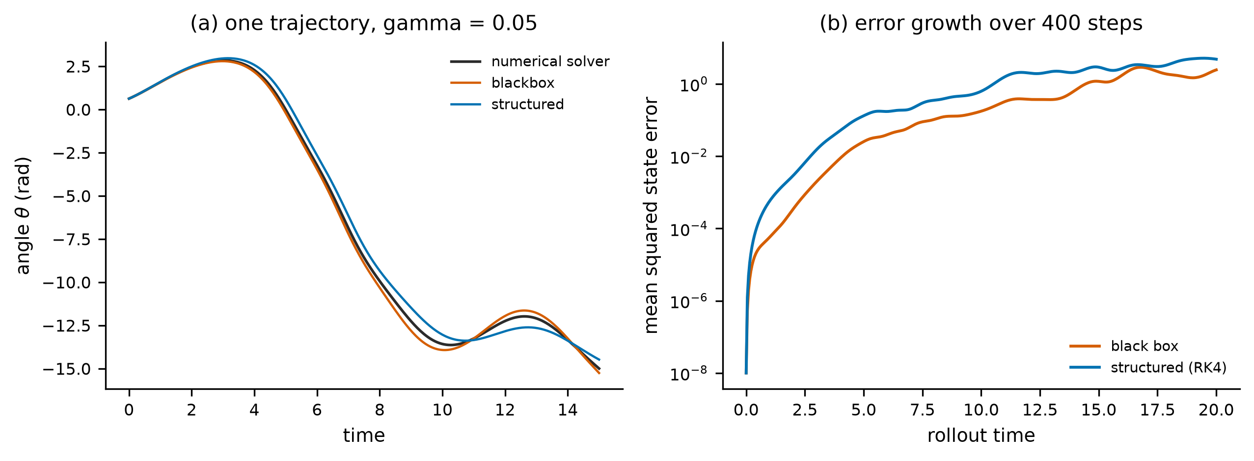
在 100 步的视界上，结果是反直觉的：黑箱模型在每一个阻尼值上都更准。

At a 100-step horizon the result is counter-intuitive: the black box is more accurate at every damping value.

阻尼 $\gamma$ / damping	黑箱 MSE / black box	结构化 MSE / structured
0.00
0.05（训练内 / in training）	0.0048	0.0251
0.15（训练外 / outside）	0.0021	0.0100
0.20（训练外 / outside）	0.0033	0.0084

English: 100-step rollout MSE (normalised by no constant; it is the raw mean squared error on $(\sin\theta,\cos\theta,\dot\theta)$).

这是我原本没有预料到的结果，也是本文刻意保留的负面结果。它说明”加入物理结构一定更好”是一个未经检验的直觉。在这个任务里，黑箱模型有更多自由度去吸收离散化误差：它预测的是 $dt$ 内的净变化，RK4 的截断误差被它顺手拟合掉了。结构化模型强制使用一个它的网络无法完全复现的积分器，反而把这部分误差留了下来。

This is the result I did not expect, and it is the negative result this article keeps on purpose. It shows that “adding physical structure always helps” is an untested intuition. Here the black box has more freedom to absorb discretisation error: it predicts the net change over $dt$, and the RK4 truncation error is fitted away with it. The structured model is forced through an integrator its network cannot reproduce exactly, and that residual stays in the prediction.

图 9　(a) 100 步 rollout 误差随阻尼的变化。训练区间是 0\le\gamma\le0.10，右侧两个柱子在训练范围之外，用作外推检验；黑箱在所有取值上都更低。 (b) 无驱动、无阻尼情形（\gamma=0，A=0，在训练集内）下 400 步内的能量误差。这一次结构化模型明显更好：它的最大能量误差只有黑箱的一半左右。 | Figure 9. (a) 100-step rollout error against damping. Training covers 0\le\gamma\le0.10; the two right-hand bars are outside the training range and serve as extrapolation tests; the black box is lower everywhere. (b) Energy error over 400 steps in the undriven, undamped case (\gamma=0, A=0, inside training). Here the structured model is clearly better: its maximum energy error is about half that of the black box. — **图 9**　(a) 100 步 rollout 误差随阻尼的变化。训练区间是 $0\le\gamma\le0.10$，右侧两个柱子在训练范围之外，用作外推检验；黑箱在所有取值上都更低。 (b) 无驱动、无阻尼情形（$\gamma=0$，$A=0$，在训练集内）下 400 步内的能量误差。这一次结构化模型明显更好：它的最大能量误差只有黑箱的一半左右。 | **Figure 9.** (a) 100-step rollout error against damping. Training covers $0\le\gamma\le0.10$; the two right-hand bars are outside the training range and serve as extrapolation tests; the black box is lower everywhere. (b) Energy error over 400 steps in the undriven, undamped case ($\gamma=0$, $A=0$, inside training). Here the structured model is clearly better: its maximum energy error is about half that of the black box.

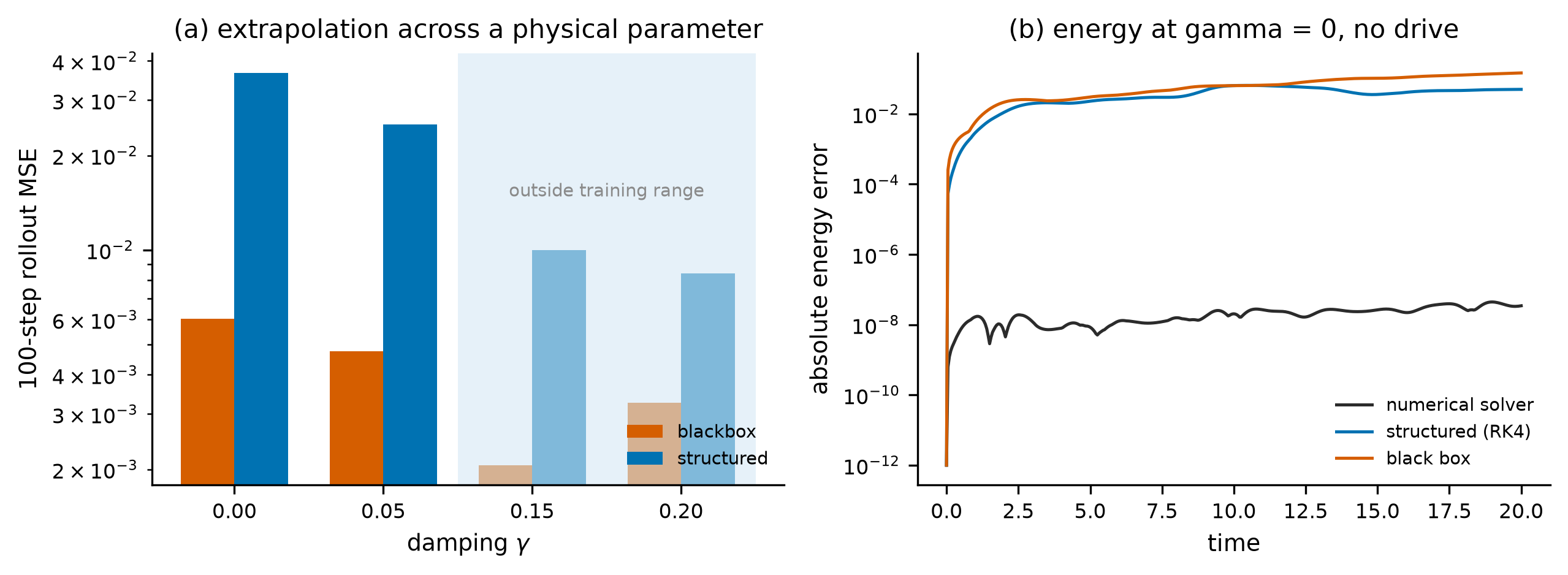
第二张图给出了另一半答案。能量 $E=\tfrac12\dot\theta^2+(1-\cos\theta)$ 在无驱动、无阻尼时应当严格守恒。黑箱模型的最大能量误差是 0.1461，结构化模型是 0.0646，数值解是 4.4e-08。没有一个模型被直接训练去守恒能量，但结构化模型因为走了一个保结构的积分器，漂移小了一半。

The second panel gives the other half. In the undriven, undamped case the energy $E=\tfrac12\dot\theta^2+(1-\cos\theta)$ should be exactly conserved. The black box’s maximum energy error is 0.1461, the structured model’s 0.0646, and the numerical solver’s 4.4e-08. Neither model was trained to conserve energy, but the structured one drifts half as much because it steps through a structure-preserving integrator.

所以结论要分成两句说：结构买不到短视界上的精度，但买得到”没被训练过的那条性质”。 对于物理系统，那条性质通常是守恒量；对于生命系统，那条性质通常是”扰动之后仍然活着”。

So the conclusion has to be split in two: structure does not buy short-horizon accuracy, but it buys a property that was never trained on. In physical systems that property is usually a conserved quantity; in living systems it is usually “still alive after the perturbation”.

4.3 混沌给所有模型设了一个上限 / Chaos sets a ceiling for every model

受迫摆在 $A=1.6$、$\gamma=0.05$ 附近是混沌的。两个初始角度相差 $10^{-3}$ 弧度的轨迹，会以指数速度分离。我们对真实系统做一个纯粹的测量（不涉及任何模型）：分离距离的对数斜率是每单位时间 0.31，也就是说误差大约每 $1/$0.31$$3.2 个时间单位放大 $e$ 倍。

The driven pendulum is chaotic near $A=1.6$, $\gamma=0.05$. Two trajectories whose initial angles differ by $10^{-3}$ radians separate exponentially. We measure this on the true system (no model involved): the log-slope of the separation is 0.31 per unit time, so errors grow by a factor of $e$ roughly every $1/$0.31$$3.2 time units.

图 10　(a) 同一条定律、两个相差 10^{-3} 弧度的初始条件，在 40 个时间单位后完全分开。 (b) 分离距离的对数坐标：它先缓慢增长，然后进入指数区，斜率约为 0.31/时间单位。任何模型，即使参数完全正确，只要初始条件有极小的误差，也会在几个 Lyapunov 时间之后失去预测能力。 | Figure 10. (a) The same law, two initial conditions 10^{-3} radians apart, fully separated after 40 time units. (b) The separation on a log scale: slow growth first, then an exponential regime with slope about 0.31 per unit time. Any model — even with exactly correct parameters — loses predictive power after a few Lyapunov times if its initial condition is slightly off. — **图 10**　(a) 同一条定律、两个相差 $10^{-3}$ 弧度的初始条件，在 40 个时间单位后完全分开。 (b) 分离距离的对数坐标：它先缓慢增长，然后进入指数区，斜率约为 0.31/时间单位。任何模型，即使参数完全正确，只要初始条件有极小的误差，也会在几个 Lyapunov 时间之后失去预测能力。 | **Figure 10.** (a) The same law, two initial conditions $10^{-3}$ radians apart, fully separated after 40 time units. (b) The separation on a log scale: slow growth first, then an exponential regime with slope about 0.31 per unit time. Any model — even with exactly correct parameters — loses predictive power after a few Lyapunov times if its initial condition is slightly off.

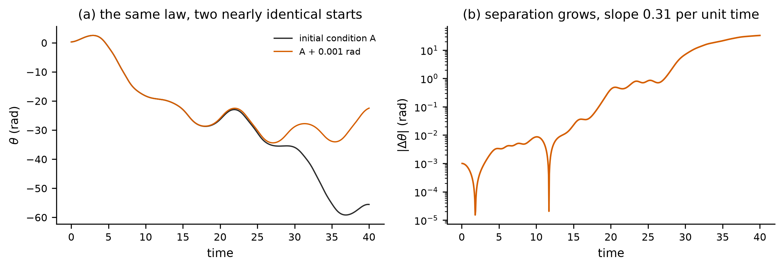
这个数字的作用是校准预期，而不是打击信心。它说：在混沌系统里，“长期精确预测”是一个数学上不可能的目标，模型能竞争的是”Lyapunov 时间之内的预测”与”统计性质（如能量、吸引子、分布）的保持”。这也解释了图 8(b) 的饱和：那不是训练不足，那是世界本身的性质。

The number calibrates expectations rather than discouraging anyone. It says that in a chaotic system “long-term accurate prediction” is a mathematically impossible target; what models can compete on is prediction within the Lyapunov time, and the preservation of statistical properties such as energy, attractors and distributions. That is also what the saturation in Figure 8b means: not insufficient training, but a property of the world.

5. 生命：自我维持的世界 / Life: the world of self-maintenance

现在到了本文的核心。前面的三个世界共享大量数学工具：状态、转移、误差、泛化。生命系统也用这些工具，但它多出几样东西——调控、代谢、适应、状态选择、多尺度组织与历史性。这一节要检验：当一个系统具备其中几样时，我们对它的建模能力会发生什么变化？

Now to the core. The first three worlds share a large mathematical toolkit: state, transition, error, generalisation. Living systems use that toolkit too, but they add regulation, metabolism, adaptation, state selection, multi-scale organisation and history. This section asks what happens to our modelling ability when a system has a few of those.

先把一句警告写在前面：非线性、涌现、自组织、混沌与反馈都不是生命的充分条件。 第 4 节的摆是非线性的、混沌的、有反馈的，它不是活的。所以本节不会用”这个系统有吸引子”来论证它是生命；我们只问一个更窄、也更可检验的问题：在一个有多个稳定状态、受环境调控、可以被敲除基因的系统上，不同建模路线在干预预测上差多少？

A warning first: nonlinearity, emergence, self-organisation, chaos and feedback are not sufficient conditions for life. The pendulum in Section 4 is nonlinear, chaotic and feedback-driven; it is not alive. So this section will not argue that a system is alive because it has attractors. It asks a narrower, testable question: on a system with several stable states, environmental regulation and knock-out perturbations, how much do modelling strategies differ when predicting interventions?

5.1 一个十基因的虚拟细胞 / A ten-gene virtual cell

模型由十个基因组成，每个基因的浓度 $x_i$ 服从激活—降解动力学：

The model has ten genes, each with activation–degradation dynamics:

\[ \frac{dx_i}{dt} = -x_i + \sum_{j} W_{ij}\,h(x_j) + b_i + u\,c_i, \qquad h(x)=\frac{x^2}{K^2+x^2} \]

其中 $W_{ij}>0$ 表示 $j$ 激活 $i$，$W_{ij}<0$ 表示抑制；$h$ 是 Hill 函数（饱和的正反馈）；$b_i$ 是基础表达；$u$ 是环境信号，$c_i$ 是基因 $i$ 对该信号的敏感度。这个方程里没有任何”细胞”：没有膜、没有代谢、没有空间。它是一个调控网络的抽象，正因为抽象，所有结论都只能停留在”调控层面”。

Here $W_{ij}>0$ means $j$ activates $i$ and $W_{ij}<0$ means inhibition; $h$ is a Hill function (saturating positive feedback); $b_i$ is basal expression; $u$ is an environmental signal and $c_i$ the sensitivity of gene $i$ to it. There is no cell in this equation: no membrane, no metabolism, no space. It is an abstraction of a regulatory network, and precisely because it is abstract, every conclusion stays at the regulatory level.

网络里有 20 条边：两个互相抑制的”开关”（$g_0\leftrightarrow g_1$ 与 $g_2\leftrightarrow g_3$），一个读取两个开关状态的枢纽基因 $g_4$，以及五个下游读出基因。

The network has 20 edges: two mutual-inhibition toggle switches ($g_0\leftrightarrow g_1$ and $g_2\leftrightarrow g_3$), a hub gene $g_4$ that reads both switches, and five downstream readouts.

图 11　网络结构。蓝线是激活，橙线是抑制（自激活为了图面清晰没有画出，但它存在于方程里）。绿色是两个开关，蓝色是枢纽，灰色是读出基因。这个结构是”先验知识”，第 5.2 节里有两个模型会拿到它，另两个不会。 | Figure 11. The network. Blue edges activate, orange edges inhibit (self-activation is omitted for legibility but is present in the equations). Green nodes are the two switches, blue is the hub, grey are readouts. This structure is prior knowledge: in Section 5.2 two models receive it and two do not. — **图 11**　网络结构。蓝线是激活，橙线是抑制（自激活为了图面清晰没有画出，但它存在于方程里）。绿色是两个开关，蓝色是枢纽，灰色是读出基因。这个结构是”先验知识”，第 5.2 节里有两个模型会拿到它，另两个不会。 | **Figure 11.** The network. Blue edges activate, orange edges inhibit (self-activation is omitted for legibility but is present in the equations). Green nodes are the two switches, blue is the hub, grey are readouts. This structure is *prior knowledge*: in Section 5.2 two models receive it and two do not.

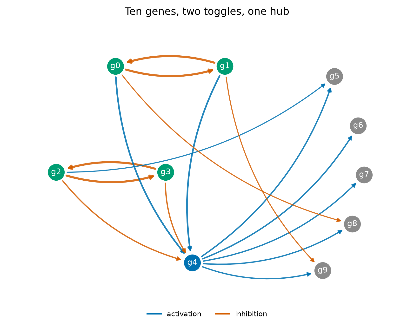
从 400 个随机初始状态出发、积分 1500 步后，系统恰好收敛到 4 个稳定状态。它们之间的差别几乎完全由两个开关的胜负决定：$g_0$ 与 $g_1$ 必有一个接近 1.66、另一个接近 0，两个开关组合出四种命运。

Starting from 400 random initial states and integrating 1500 steps, the system settles into exactly 4 stable states. The differences are almost entirely decided by which side wins each toggle: one of $g_0,g_1$ sits near 1.66 and the other near 0, and the two switches combine into four fates.

图 12　同一段环境信号，两个不同的起点。(a) 细胞 A 从”开关 A 关闭”的状态出发：信号持续 30 个时间单位，g_0 被释放、g_1 被压下去；信号撤去之后，g_0 保持在 1.66——这是一次不可逆的状态切换。 (b) 细胞 B 从”开关 A 已开”的状态出发，同一个信号几乎没有留下痕迹。 | Figure 12. The same environmental signal, two different starting states. (a) Cell A starts with toggle A off: the signal lasts 30 time units, g_0 is released and g_1 is suppressed; after the signal is removed g_0 stays at 1.66 — an irreversible state switch. (b) Cell B starts with toggle A already on, and the same signal leaves almost no trace. — **图 12**　同一段环境信号，两个不同的起点。(a) 细胞 A 从”开关 A 关闭”的状态出发：信号持续 30 个时间单位，$g_0$ 被释放、$g_1$ 被压下去；信号撤去之后，$g_0$ 保持在 1.66——**这是一次不可逆的状态切换**。 (b) 细胞 B 从”开关 A 已开”的状态出发，同一个信号几乎没有留下痕迹。 | **Figure 12.** The same environmental signal, two different starting states. (a) Cell A starts with toggle A off: the signal lasts 30 time units, $g_0$ is released and $g_1$ is suppressed; after the signal is removed $g_0$ stays at 1.66 — **an irreversible state switch**. (b) Cell B starts with toggle A already on, and the same signal leaves almost no trace.

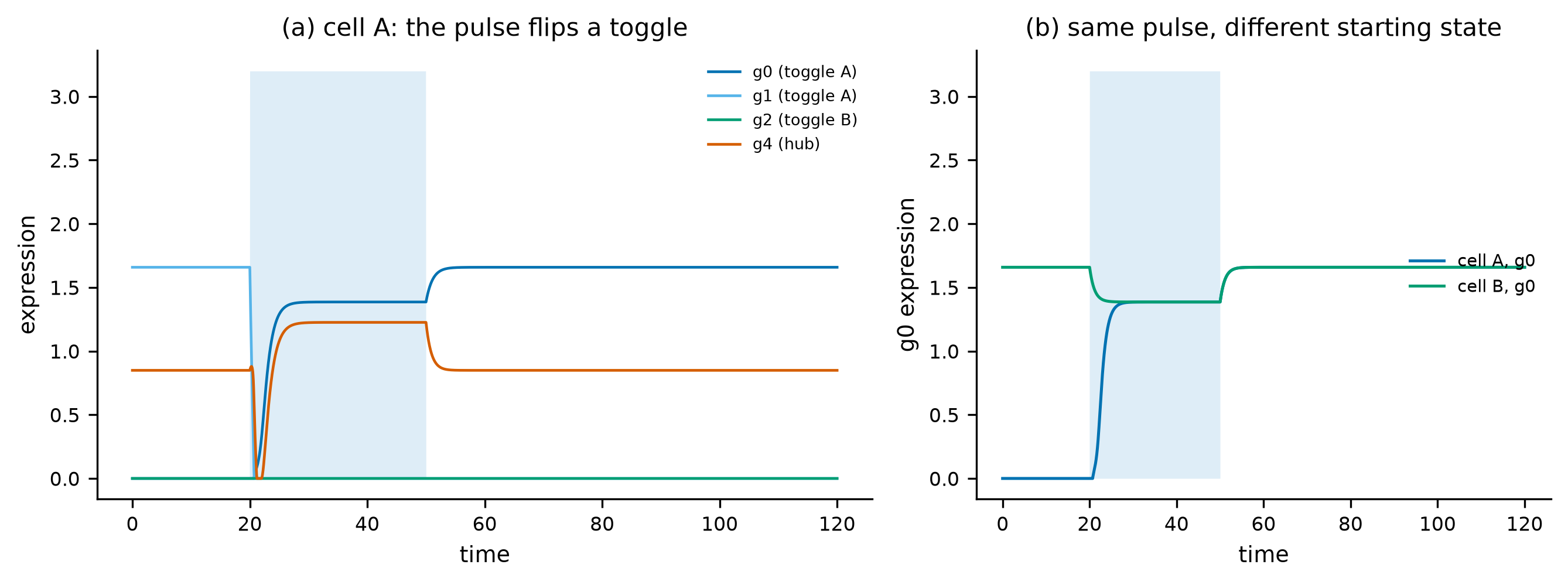
这张图里藏着本文关于”细胞”的第一条实质结论：同一个扰动，结果取决于细胞处在哪个状态。 细胞 A 与细胞 B 面对完全相同的信号、相同的网络、相同的参数，一个被永久改写，一个毫无变化。任何只以”扰动”为输入、不以”状态”为输入的预测模型，在这种系统上必然出错——因为它的输入里缺少了决定结果的那个变量。

The figure contains the first substantive claim about cells: the same perturbation has a different outcome depending on the state the cell is in. Cells A and B face the same signal, the same network and the same parameters; one is permanently rewritten, the other is untouched. Any predictor whose input is only the perturbation, and not the state, must fail on such a system — the variable that decides the outcome is missing from its input.

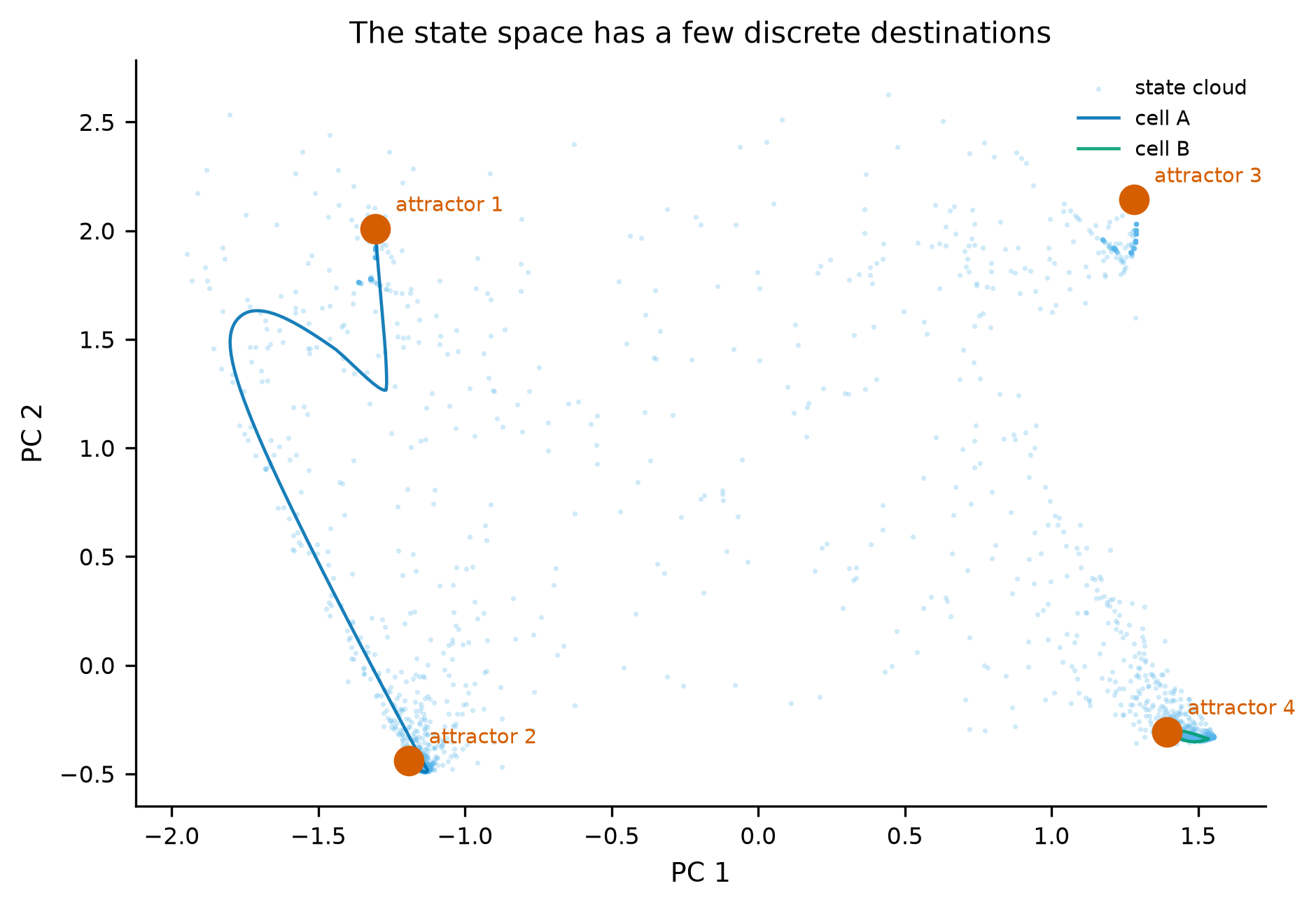
图 13　状态空间（前两个主成分，解释 61% 与 25% 的方差）。浅蓝点是 260 条随机轨迹上的状态采样，红点是 4 个吸引子，两条彩线是图 12 中两个细胞的实际轨迹。 | Figure 13. State space (first two principal components, explaining 61% and 25% of the variance). Pale blue points are states sampled from 260 random trajectories, red dots are the 4 attractors, and the two coloured lines are the actual trajectories of the cells in Figure 12. — **图 13**　状态空间（前两个主成分，解释 61% 与 25% 的方差）。浅蓝点是 260 条随机轨迹上的状态采样，红点是 4 个吸引子，两条彩线是图 12 中两个细胞的实际轨迹。 | **Figure 13.** State space (first two principal components, explaining 61% and 25% of the variance). Pale blue points are states sampled from 260 random trajectories, red dots are the 4 attractors, and the two coloured lines are the actual trajectories of the cells in Figure 12.

我们还做了一次”上扫—下扫”实验：把信号从 0 缓慢升到 2，再从 2 降回 0，每一步都让系统重新稳定。如果系统是简单的输入—输出函数，两条路径应当重合；实际上两条路径在开关状态上最多相差 1.66。这是迟滞（hysteresis）：系统记住了自己是怎么来的。 记忆不是被存进某个变量里的，而是被存在吸引子的选择里。

We also ran an up-and-down sweep: raise the signal slowly from 0 to 2, then lower it back to 0, letting the system settle at each step. If the system were a simple input–output function the two paths would coincide; in fact they differ by up to 1.66 in toggle state. This is hysteresis: the system remembers how it got here. The memory is not stored in a variable; it is stored in the choice of attractor.

5.2 从观测到干预 / From observation to intervention

现在做实验 5.2：训练四个模型预测基因敲除之后的细胞状态。这是一个比”预测下一帧”更严格的测试，因为敲除改变了系统本身，而不只是它的初始条件。

Now experiment 5.2: four models are trained to predict the cell state after a gene knockout. This is stricter than “predict the next frame”, because a knockout changes the system, not just its initial condition.

数据：3,000 条轨迹，每条 20 步。训练集只包含基因 $g_0,g_1,g_2$ 的单基因敲除，环境为 $u\in\{0,1\}$。测试集刻意向外推：未敲除过的基因 $g_3,g_4$、双基因敲除、以及训练中没出现过的环境 $u=0.5$ 与 $u=1.5$。

Data: 3,000 trajectories of 20 steps. Training contains only single knockouts of genes $g_0,g_1,g_2$, under environments $u\in\{0,1\}$. The tests move outwards on purpose: genes never knocked out ($g_3,g_4$), double knockouts, and environments absent from training ($u=0.5$, $u=1.5$).

四个模型，信息量刻意做成阶梯：

Four models, with a deliberate ladder of information:

模型 / Model	输入 / Inputs	是否知道网络 / Knows the graph
持续性 / persistence	当前状态 / current state	否 / no
MLP	当前状态 + 敲除 + 环境 / state + KO + env	否 / no
图网络 / graph net	同上，但通过 $W$ 做邻域聚合 / same, aggregated through $W$	是 / yes
机理拟合 / mechanistic	同一族 ODE，固定 $W$，拟合常数 / same ODE family, fixed $W$, fitted constants	是 / yes

要诚实说明：图网络与机理模型拿到的是先验优势，不是它们自己发现的规律。这不是不公平，而是本文想量化的东西——“已知结构”在干预预测上值多少。

Honesty requires saying that the graph network and the mechanistic model receive a prior advantage; they did not discover the structure. That is not unfair, it is the quantity being measured: what is prior knowledge worth for intervention prediction?

图 14　(a) 20 步后的预测误差（以响应方差归一化，对数纵轴）。 (b) 方向正确率：对每个显著变化的基因，预测的变化方向对不对。持续性模型在 (b) 中低于 0.5，因为它把”不变”当作答案，凡是真实发生变化的基因都被判错。 | Figure 14. (a) Prediction error after 20 steps, normalised by the response variance (log scale). (b) Direction accuracy: for every gene that changes substantially, did the model get the sign right? Persistence falls below 0.5 in (b) because it predicts “no change”, and every gene that actually moves is counted wrong. — **图 14**　(a) 20 步后的预测误差（以响应方差归一化，对数纵轴）。 (b) 方向正确率：对每个显著变化的基因，预测的变化方向对不对。持续性模型在 (b) 中低于 0.5，因为它把”不变”当作答案，凡是真实发生变化的基因都被判错。 | **Figure 14.** (a) Prediction error after 20 steps, normalised by the response variance (log scale). (b) Direction accuracy: for every gene that changes substantially, did the model get the sign right? Persistence falls below 0.5 in (b) because it predicts “no change”, and every gene that actually moves is counted wrong.

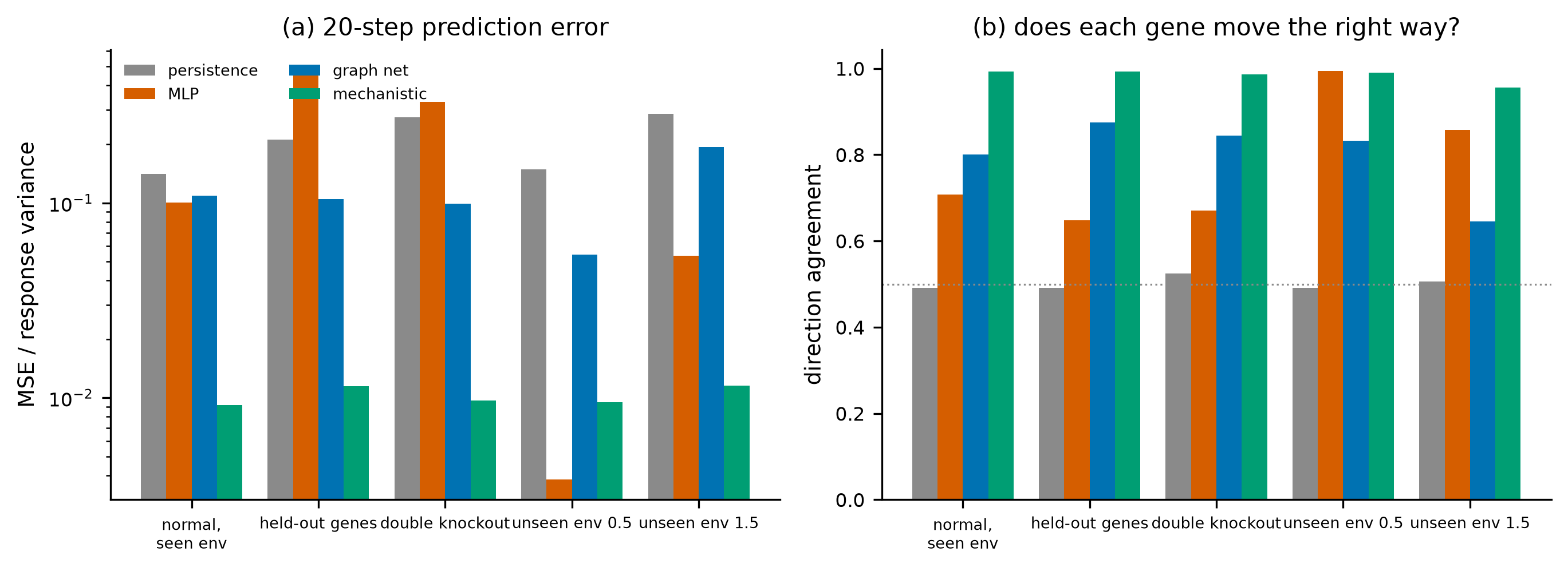
结果分成三块，每一块都值得单独说。

The results fall into three blocks, each worth stating separately.

第一块是分布内。正常状态下，MLP 的误差是 0.100，图网络是 0.109：两者几乎一样。这符合直觉——数据覆盖了这种情形，结构没有额外信息可提供。

The first block is in-distribution. In the normal state the MLP has error 0.100 and the graph network 0.109: essentially the same. That is expected — the data cover this case, so structure adds nothing.

第二块是新的干预。敲除从未敲除过的基因 $g_3$ 或 $g_4$ 时，MLP 的误差涨到 0.479，比持续性基线（0.211）还差；图网络保持在 0.104。双敲除上差距更大：MLP 0.329，图网络 0.099。方向正确率也分开了：双敲除时图网络 84.4%，MLP 67.1%。

The second block is new interventions. Knocking out genes never knocked out before ($g_3$ or $g_4$), the MLP’s error rises to 0.479, worse than the persistence baseline (0.211); the graph network stays at 0.104. The gap widens for double knockouts: MLP 0.329, graph network 0.099. Direction accuracy separates too: 84.4% versus 67.1%.

图 15　一次双基因敲除（g_2 与 g_4）之后的真实状态与两个模型的预测。g_1 从被抑制变为高表达，g_4 被敲除，g_5 与下游读出随之上调。图网络在这些基因上明显更接近真实值；MLP 系统性地高估了 g_1 的响应。 | Figure 15. True state after a double knockout of g_2 and g_4, together with two models’ predictions. g_1 goes from suppressed to high, g_4 is absent, and g_5 plus the readouts rise accordingly. The graph network is visibly closer on those genes; the MLP systematically overestimates the response of g_1. — **图 15**　一次双基因敲除（$g_2$ 与 $g_4$）之后的真实状态与两个模型的预测。$g_1$ 从被抑制变为高表达，$g_4$ 被敲除，$g_5$ 与下游读出随之上调。图网络在这些基因上明显更接近真实值；MLP 系统性地高估了 $g_1$ 的响应。 | **Figure 15.** True state after a double knockout of $g_2$ and $g_4$, together with two models’ predictions. $g_1$ goes from suppressed to high, $g_4$ is absent, and $g_5$ plus the readouts rise accordingly. The graph network is visibly closer on those genes; the MLP systematically overestimates the response of $g_1$.

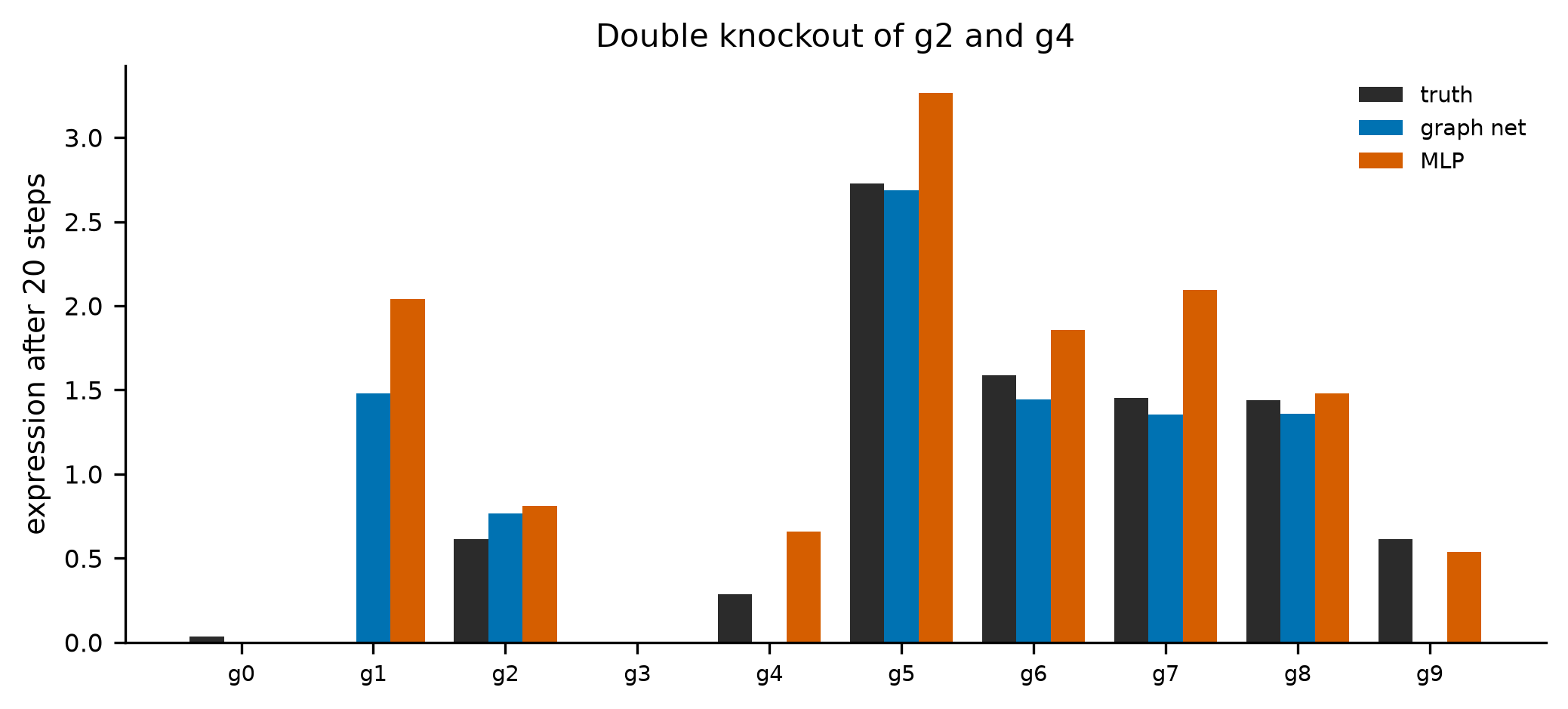
第三块是长期。这一块是反过来的：在 200 步之后，MLP 的误差是 0.118，图网络是 0.845，机理模型是 0.676，持续性基线是 0.841。在长视界上，反而是 MLP 最好，两个”懂结构”的模型都输给了持续性基线。

The third block is the long horizon, and it reverses the picture: after 200 steps the MLP’s error is 0.118, the graph network 0.845, the mechanistic model 0.676, and persistence 0.841. At long horizons the MLP wins, and both “structure-aware” models lose even to the persistence baseline.

这个结果需要解释，而不是掩饰。长视界的误差主要由吸引子的位置决定：系统最终停在哪一个稳定状态、停得多准。MLP 训练时见过大量”停稳之后”的状态，它记住了这些吸引子的位置；机理模型的参数只是拟合到近似正确，参数上的小偏差会把吸引子挪动一点，而这一点位移在 200 步之后被完整地暴露出来。“一步很准”与”最终停对地方”是两个不同的目标，前者靠结构，后者靠见过。

The result needs explanation, not concealment. Long-horizon error is dominated by where the attractor is: which stable state the system ends in, and how accurately. The MLP saw many settled states during training and memorised their positions; the mechanistic model’s parameters are only approximately right, and a small parameter error shifts the attractor slightly — a displacement fully exposed after 200 steps. “Accurate one step ahead” and “ends up in the right place” are different objectives: the first favours structure, the second favours having seen it.

5.3 结构值多少：一个故意的破坏实验 / What structure is worth: a deliberate damage test

为了不把”结构有用”变成一个无法反驳的口号，我们做了一次破坏实验：把真实网络中 30% 的边（20 条中的 6 条）随机删掉，再用同样的方式训练图网络。

To keep “structure helps” from becoming an unfalsifiable slogan, we ran a damage test: delete 30% of the edges in the true network at random (6 of 20), then train the graph network in exactly the same way.

图 16　双敲除预测误差：完整图网络、被删掉 30% 边的图网络、以及 MLP。结构被破坏之后，图网络的优势明显缩小，但仍好于纯数据模型。这说明它的收益来自具体的边，而不是”多了一个模块”。 | Figure 16. Double-knockout prediction error for the full graph network, the network with 30% of its edges removed, and the MLP. After the damage the graph model’s advantage shrinks markedly, though it remains better than the pure data model. The benefit comes from specific edges, not from having an extra module. — **图 16**　双敲除预测误差：完整图网络、被删掉 30% 边的图网络、以及 MLP。结构被破坏之后，图网络的优势明显缩小，但仍好于纯数据模型。这说明它的收益来自**具体的边**，而不是”多了一个模块”。 | **Figure 16.** Double-knockout prediction error for the full graph network, the network with 30% of its edges removed, and the MLP. After the damage the graph model’s advantage shrinks markedly, though it remains better than the pure data model. The benefit comes from **specific edges**, not from having an extra module.

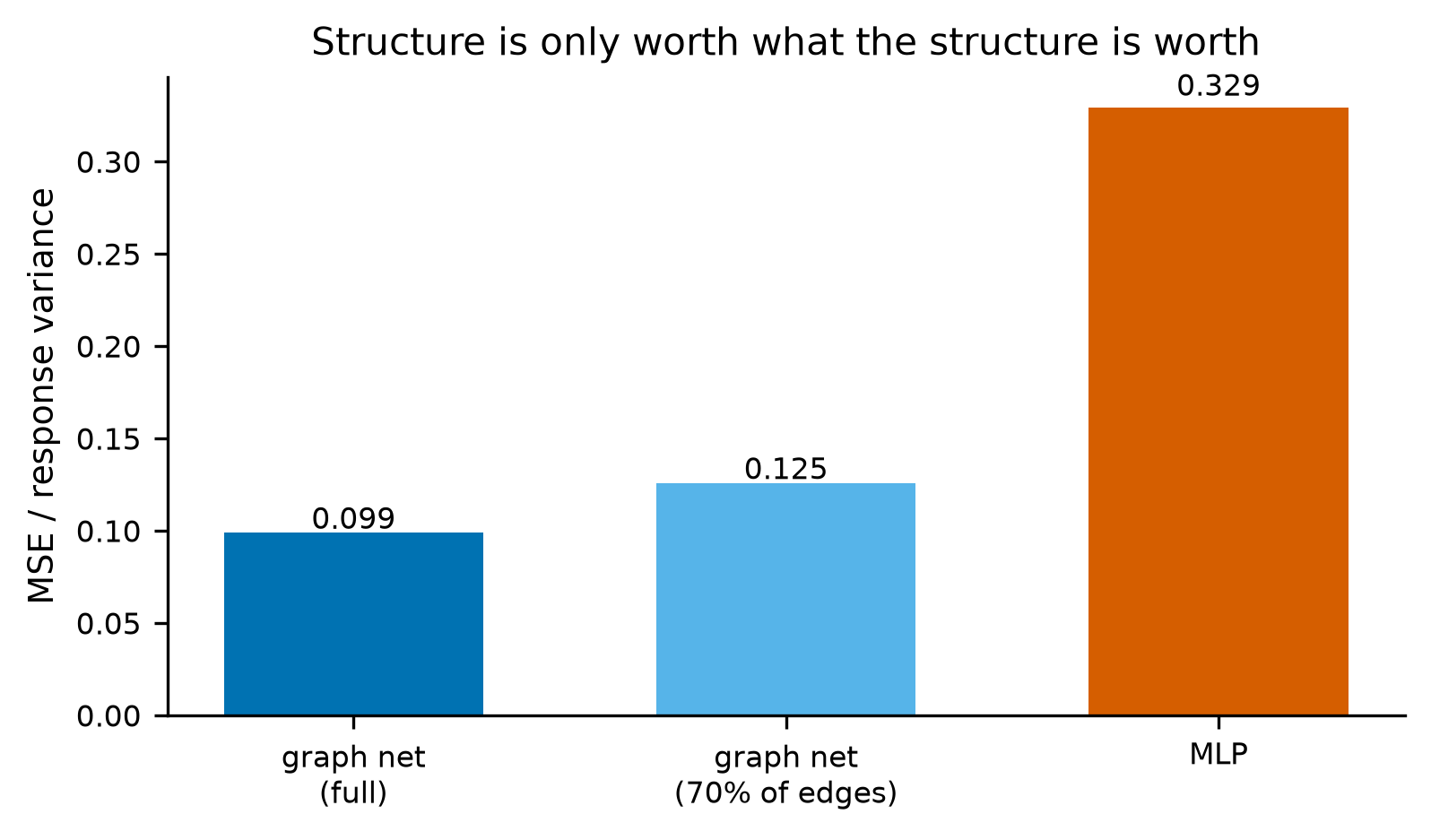
完整图网络的误差是 0.099，损坏后是 0.126，MLP 是 0.329。三个数字排成一条线：结构有用，但用的是”正确的结构”。 一个错误的结构仍然比没有结构好一点——它会给出一个合理的先验形状——但它买不回全部收益。

The full graph network has error 0.099, the damaged one 0.126, and the MLP 0.329. Three numbers in a line: structure helps, but only the right structure. A wrong structure is still somewhat better than none — it supplies a plausible prior shape — but it does not recover the full benefit.

5.4 这一节没有做的事 / What this section did not do

有三件事被刻意留在了外面，必须说清楚，否则上面的结论会被读得过宽。

Three things were deliberately left out, and saying so matters, otherwise the conclusions above will be read too broadly.

第一，没有进化。真正的生命系统会变异、复制、被选择；我们的细胞不会。加入一个简化的复制—变异—选择循环并不困难（一个准物种方程就够），但那会引入”适应度函数是人为设定的”这一层新的不诚实：自然选择没有一个写在纸上的目标函数，而任何模拟都必须写一个。这个矛盾本身值得单独一篇文章。

First, no evolution. Real living systems mutate, replicate and are selected; our cell does none of that. Adding a simplified replicate–mutate–select loop is not hard (a quasispecies equation would do), but it introduces a new layer of dishonesty: the fitness function is written by us, whereas natural selection has no objective function on paper. That tension deserves its own article.

第二，没有代谢。我们的”细胞”不消耗能量、不产生废物、不维持一个远离平衡的内部环境。它的稳定性来自方程的吸引子，而不是来自持续的能量输入。这是玩具模型与真实细胞之间最大的鸿沟之一：真实细胞的稳定是耗能的稳定，一旦停止供能就崩溃；我们的模型即使”断电”也会安静地待着。

Second, no metabolism. Our “cell” consumes no energy, produces no waste and maintains no out-of-equilibrium interior. Its stability comes from attractors in the equations, not from a continuous energy flux. That is one of the largest gaps to a real cell: real stability is paid for with energy and collapses when supply stops; our model would sit quietly even after the power was cut.

第三，没有空间。真实的细胞有几何、有区室、有极性；我们的十个基因住在一个充分混合的试管里。空间只有在反应—扩散模型里才会出现，而那是另一个尺度的问题。

Third, no space. Real cells have geometry, compartments and polarity; our ten genes live in a well-mixed test tube. Space only enters in reaction–diffusion models, which are a different scale of problem.

即便如此，这一节的结论仍然成立，因为它只声称一件事：在一个多稳态、可被干预的调控系统上，“知道结构”与”只看到数据”在面对新干预时表现出可测量的差别，而这种差别在长视界上会反号。 这句话既不夸张，也不空洞，而且它可以被任何人在 CPU 上重跑。

Even so, the conclusions hold, because they claim only one thing: on a multi-stable, intervenable regulatory system, “knowing the structure” and “only seeing data” differ measurably on new interventions, and that difference reverses sign at long horizons. The claim is neither inflated nor empty, and anyone can rerun it on a CPU.

6. 四个世界的共同数学 / The mathematics the four worlds share

把四组实验写成同一行，会得到一件有用的东西，也会得到一件危险的东西。有用的东西是一个统一的分析语言：

Writing the four experiments in one line gives something useful and something dangerous. The useful thing is a common analytical language:

\[ x(t+1) = F\big(x(t),\,u(t),\,e(t),\,\theta\big) \]

$x$ 是状态，$u$ 是输入或干预，$e$ 是环境，$\theta$ 是参数。这个形式对四个世界都成立：语言里 $x$ 是已生成的词序列、$u$ 是提示、$\theta$ 是权重；图像里 $x$ 是像素或潜在编码、$u$ 是条件；物理里 $x=(\theta,\dot\theta)$、$u$ 是外力、$\theta$ 是阻尼与驱动幅度；虚拟细胞里 $x$ 是十个基因的浓度、$u$ 是信号、$\theta$ 是调控强度。

$x$ is the state, $u$ an input or intervention, $e$ the environment, $\theta$ the parameters. The form holds for all four worlds: in language $x$ is the generated token sequence, $u$ a prompt, $\theta$ the weights; in images $x$ is pixels or a latent code, $u$ a conditioning signal; in physics $x=(\theta,\dot\theta)$, $u$ an external force, $\theta$ the damping and drive; in the virtual cell $x$ is ten concentrations, $u$ the signal, $\theta$ the regulatory strengths.

危险的东西是：这个统一只是记号上的统一。 同一个方程形式，四个世界里的 $F$ 性质完全不同——语言的 $F$ 是离散的、有长程依赖的；图像的 $F$ 作用在一个低维流形上；物理的 $F$ 有守恒律与时间可逆性；生命的 $F$ 有多个吸引子，而且 $\theta$ 本身会随历史改变。把它们写成同一行，不会让它们变成同一个问题。

The dangerous thing is that the unification is notational only. The same equation form hides four very different $F$’s: in language it is discrete and long-range; in images it acts on a low-dimensional manifold; in physics it obeys conservation laws and time reversibility; in life it has several attractors, and $\theta$ itself changes with history. Writing them in one line does not make them one problem.

图 17　跨领域比较（作者的主观评分，1–3，不是测量值）。行是十二个难度维度，列是四个世界。它的用途不是”证明生命最难”，而是指出难度来自不同的行：生命的难点集中在反馈、干预、因果可识别性、多尺度与历史；物理的难点集中在长视界与混沌；语言与图像的难点更多在分布偏移与评价标准。 | Figure 17. Cross-domain comparison (the author’s qualitative rating, 1–3; not a measurement). Rows are twelve dimensions of difficulty, columns the four worlds. Its purpose is not to prove that life is hardest, but to show that the difficulty comes from different rows: life’s difficulties cluster in feedback, intervention, causal identifiability, multi-scale organisation and history; physics’ in long horizons and chaos; language and images in distribution shift and evaluation. — **图 17**　跨领域比较（作者的主观评分，1–3，不是测量值）。行是十二个难度维度，列是四个世界。它的用途不是”证明生命最难”，而是指出**难度来自不同的行**：生命的难点集中在反馈、干预、因果可识别性、多尺度与历史；物理的难点集中在长视界与混沌；语言与图像的难点更多在分布偏移与评价标准。 | **Figure 17.** Cross-domain comparison (the author’s qualitative rating, 1–3; not a measurement). Rows are twelve dimensions of difficulty, columns the four worlds. Its purpose is not to prove that life is hardest, but to show that **the difficulty comes from different rows**: life’s difficulties cluster in feedback, intervention, causal identifiability, multi-scale organisation and history; physics’ in long horizons and chaos; language and images in distribution shift and evaluation.

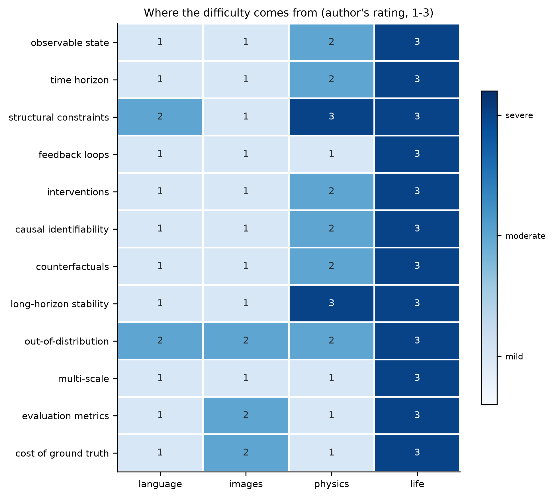
这张图必须配一句免责声明：格子里的数字是我的判断，不是实验输出。 它可以被质疑，也应该被质疑；它的价值在于把”哪个领域更难”这个笼统的问题拆成十二个可以分别争论的问题。其中三行在本文的实验里都有直接读数：因果可识别性对应第 5 节的新干预测试（“改变一个基因之后会发生什么”是 $do$ 问题，不是相关问题）；分布外泛化对应第 2 节的长距离一致率与分布外比特数；评价指标对应第 2 节结尾那句”损失低不等于理解”。

The figure needs a disclaimer: the numbers in the cells are my judgement, not experimental output. They can and should be contested; their value is to split the vague question “which domain is harder” into twelve questions that can be argued separately. Three of the rows have direct readings in this article’s experiments: causal identifiability corresponds to Section 5’s new-intervention tests (“what happens after I change a gene” is a $do$ question, not a correlational one); out-of-distribution generalisation to the long-distance agreement and OOD bits of Section 2; and evaluation metrics to the closing line of Section 2, “low loss is not understanding”.

另外三行只有部分实验支撑，而且支撑方式不同。第一行是隐藏状态：语言与图像的输入几乎就是全部可观测量，物理的 $\dot\theta$ 已经需要估计，细胞的浓度在真实实验里只能通过测序间接观测。第二行是干预：第 5 节的数字显示，同一个模型在”看”与”做”上的表现差距可以达到一个数量级（MLP 在分布内 0.100，在新干预上 0.329）。第三行是长视界：物理的混沌与细胞的多稳态都会让长视界预测失效，但失效的机制不同——前者是误差放大，后者是吸引子选错。

Three further rows have only partial experimental support, and in different forms. The first is hidden state: in language and images the input is nearly all there is to observe; in physics $\dot\theta$ already has to be estimated; in a cell the concentrations are only indirectly observable through sequencing. The second is intervention: Section 5 shows that the same model can differ by an order of magnitude between “seeing” and “doing” (MLP 0.100 in-distribution versus 0.329 on a new intervention). The third is long horizon: chaos in physics and multi-stability in cells both break long-horizon prediction, but by different mechanisms — error amplification versus choosing the wrong attractor.

7. 为什么生命模拟可能是 AI 的圣殿 / Why life simulation may be AI’s sanctuary

现在可以正面回答标题了。我要给出的不是一个”生命最复杂”的断言，而是九个具体的、可以分别检验的理由；然后给出一个反对意见，并说明它为什么不能推翻结论。

The title can now be answered directly. What follows is not the assertion that “life is the most complex”, but nine specific and separately checkable reasons; then an objection, and why it does not overturn the conclusion.

多尺度耦合。一个细胞里同时发生着毫秒级的构象变化、分钟级的信号传导、小时级的细胞周期与天级的谱系决定。这四层互相约束，不能分别建模再拼起来。
Multi-scale coupling: conformational changes at milliseconds, signalling at minutes, the cell cycle at hours and lineage decisions at days all constrain one another; they cannot be modelled separately and then glued together.
关键状态不可直接观测。我们测到的是 RNA 计数，想要的是调控状态；从观测到状态是一次没有唯一答案的反演。
Key states are not directly observable: we measure RNA counts and want regulatory state; the map from one to the other is an inversion with no unique answer.
强烈的条件依赖性。第 5 节的图 12：同一个信号，两个起点，两种命运。这不是噪声，这是系统的结构。
Strong context dependence: Figure 12 of Section 5 — one signal, two starting states, two fates. That is not noise, it is the structure of the system.
相关不等于因果。表达相关的两个基因，可能一个是另一个的下游，也可能都被第三个基因控制；不做干预无法区分。
Correlation is not causation: two co-expressed genes may be upstream and downstream, or both controlled by a third; without intervention they cannot be told apart.
同一个干预在不同状态上给出不同结果，因此”平均处理效应”在细胞层面经常是误导性的统计量。
The same intervention gives different outcomes in different states, so the “average treatment effect” is often a misleading statistic at the cellular level.
泛化要求跨越环境、状态乃至物种。一个在小鼠肝脏上训练的模型，凭什么预测人类神经元？
Generalisation must cross environments, states and even species. Why should a model trained on mouse liver predict a human neuron?
真值昂贵且有偏。一次 Perturb-seq 实验的成本、批次效应与筛选偏差，都会进入训练数据，并被模型当作生物学学习。
Ground truth is expensive and biased: the cost, batch effects and selection bias of a Perturb-seq experiment all enter the training data and are learned as if they were biology.
历史性与开放式复杂。进化没有目标函数，生命系统的许多特征不是”最优解”，而是”路径的残留”。
Historicity and open-ended complexity: evolution has no objective function, and many features of living systems are residues of a path rather than optima.
科学价值取决于可检验的新预测。一个虚拟细胞如果只能复现已知现象，它对科学没有贡献；它必须能提出一个此前没人想到、并且可以被实验证伪的预测。
Scientific value depends on testable new predictions: a virtual cell that only reproduces what is already known contributes nothing; it must propose something nobody has thought of, which an experiment can falsify.

这九条里，没有一条是生命独有的。多尺度耦合出现在气候里，隐藏状态出现在量子力学里，昂贵真值出现在粒子物理里，历史性出现在宇宙学里。所以”生命最难”不能作为一个先验命题。

None of the nine is unique to life. Multi-scale coupling appears in climate, hidden state in quantum mechanics, expensive ground truth in particle physics, historicity in cosmology. So “life is hardest” cannot be a premise.

反对意见因此很自然：湍流的三维 Navier–Stokes 方程至今没有一般的正则性结果；多体量子系统的态空间维数随粒子数指数增长；整个宇宙的模拟在信息论意义上是不可能的。这些问题的复杂度不低于生命，甚至更高。如果”圣殿”指的是”最难”，那生命模拟排不上第一。

The objection follows naturally: the three-dimensional Navier–Stokes equations still lack a general regularity result; the state space of a many-body quantum system grows exponentially with particle number; simulating the entire universe is information-theoretically impossible. These are no less complex than life, perhaps more so. If “sanctuary” means “hardest”, life simulation does not take first place.

这个反对意见是对的，而且它逼出了标题的准确含义。生命模拟之所以是”圣殿”，不是因为它单项最难，而是因为它是唯一一个把”预测、机制、干预、多尺度、长期适应”五项要求同时压在同一张实验台上的领域。在语言里，你可以只要预测，不要机制；在物理里，你可以只要机制，不要适应；在图像里，你可以只要分布，不要干预。生命不给你这个选择：一个不能预测新干预的模型不是虚拟细胞；一个不能解释机制的模型不是科学；一个不能跨越状态与环境的模型没有用处。

The objection is correct, and it forces the precise meaning of the title. Life simulation is a “sanctuary” not because it is the hardest on any single axis, but because it is the only field that puts prediction, mechanism, intervention, multi-scale organisation and long-term adaptation on the same bench at the same time. In language you can have prediction without mechanism; in physics, mechanism without adaptation; in images, a distribution without intervention. Life does not offer that choice: a model that cannot predict new interventions is not a virtual cell; one that cannot explain a mechanism is not science; one that cannot cross states and environments is not useful.

用一句更谨慎的话说：生命模拟不是复杂度的高峰，而是约束的交点。 这正是”圣殿”这个词在科学上应该有的意思——不是最难爬的山，而是所有路都必须经过的那个地方。

Put more carefully: life simulation is not the peak of complexity, it is the intersection of constraints. That is what “sanctuary” should mean scientifically — not the hardest mountain, but the place every road has to pass through.

8. 虚拟细胞与下一代 AI / Virtual cells and the next generation of AI

如果把第 7 节的九条要求放到当前的技术版图上，会看到一个很清楚的分工：不同的模型在不同的行上得分，没有一个模型在所有行上得分。

Putting the nine requirements of Section 7 onto today’s technical map reveals a clear division of labour: different models score on different rows, and none scores on all of them.

结构预测已经接近解决，但它不是虚拟细胞。 AlphaFold 2（2021）把蛋白质从序列到结构的预测误差降到了实验精度附近，AlphaFold 3（2024）把范围扩展到复合物与小分子。这是真实的、巨大的进步。但一个蛋白质的结构不等于一个细胞的状态：AlphaFold 不模拟表达、不模拟调控、不模拟时间。把它当作虚拟细胞，是这一类讨论里最常见的范畴错误。

Structure prediction is close to solved, but it is not a virtual cell. AlphaFold 2 (2021) brought sequence-to-structure prediction close to experimental accuracy, and AlphaFold 3 (2024) extended the scope to complexes and small molecules. That is real and enormous progress. But a protein’s structure is not a cell’s state: AlphaFold does not model expression, regulation or time. Treating it as a virtual cell is the most common category error in these discussions.

基因组调控正在被大规模序列模型接管。 AlphaGenome（2025 年发布，2026 年发表于 Nature）用一条 DNA 序列同时预测数千条调控轨道，并据此评估变异的影响。它处理的是”序列到调控活性”的映射，仍然不是”细胞状态随时间的演化”，但它把”隐藏状态”这一行往前推了一大步。

Genomic regulation is being taken over by large sequence models. AlphaGenome (announced 2025, published in Nature in 2026) predicts thousands of regulatory tracks from a single DNA sequence and uses them to score variants. It models sequence-to-activity, not the evolution of cell state in time, but it moves the “hidden state” row forward substantially.

单细胞基础模型与扰动预测是离”虚拟细胞”最近的一类工作。 Geneformer、scGPT 一类模型在千万级细胞图谱上预训练，把细胞当作 token 序列；GEARS 用基因图结构预测未见过的多基因扰动；CellOT 用神经最优传输学习扰动引起的分布移动。Arc Institute 的 STATE 走的是另一条路：把”状态嵌入”与”状态转移”分成两个模块，前者学细胞的表示，后者学扰动之后状态如何移动。2025 年 6 月，Arc 发起了首届 Virtual Cell Challenge，把”在未见的细胞类型（H1 人类胚胎干细胞）上预测扰动效应”做成公开基准，前三名奖金分别为 10 万、5 万与 2.5 万美元。

Single-cell foundation models and perturbation prediction are the closest work to a “virtual cell”. Models such as Geneformer and scGPT are pretrained on atlases of tens of millions of cells, treating a cell as a token sequence; GEARS uses a gene graph to predict unseen multi-gene perturbations; CellOT uses neural optimal transport to learn the distribution shift a perturbation induces. Arc Institute’s STATE takes another route, splitting “state embedding” from “state transition”: the first learns a representation of the cell, the second learns how the state moves after a perturbation. In June 2025 Arc launched the first Virtual Cell Challenge, making “predict perturbation effects in an unseen cell type (H1 human embryonic stem cells)” a public benchmark, with first, second and third prizes of $100k, $50k and $25k.

这些工作的共同点值得注意：没有一个是纯粹的”大模型”路线。 GEARS 依赖基因图，CellOT 依赖最优传输的几何，STATE 依赖”嵌入 + 转移”的分解，机理模型依赖 ODE。第 5 节的实验给出了一个微观版本的同一条教训：MLP 在分布内最好，图网络在新干预上最好，机理模型在守恒量上最好。未来的虚拟细胞大概率是组合体，而不是一个万能模型。

One common feature deserves attention: none of these is a pure “big model” route. GEARS relies on a gene graph, CellOT on the geometry of optimal transport, STATE on an embedding-plus-transition decomposition, mechanistic models on ODEs. Section 5 gives a microscopic version of the same lesson: the MLP is best in-distribution, the graph network on new interventions, the mechanistic model on conserved quantities. The virtual cell of the future is likely a composite, not a single universal model.

图 18　Predict → Explain → Design → Validate。这四个环节构成一个闭环：预测必须落在没见过的干预上，解释必须给出机制而不只是拟合，设计必须选择下一个信息量最大的实验，验证必须回到湿实验或新的模拟。闭环转不起来，“虚拟细胞”就只是一个预测器。 | Figure 18. Predict → Explain → Design → Validate. The four steps form a loop: prediction must land on unseen interventions, explanation must give a mechanism rather than a fit, design must choose the next most informative experiment, and validation must return to the wet lab or a new simulation. If the loop does not turn, a “virtual cell” is only a predictor. — **图 18**　Predict → Explain → Design → Validate。这四个环节构成一个闭环：预测必须落在没见过的干预上，解释必须给出机制而不只是拟合，设计必须选择下一个信息量最大的实验，验证必须回到湿实验或新的模拟。闭环转不起来，“虚拟细胞”就只是一个预测器。 | **Figure 18.** Predict → Explain → Design → Validate. The four steps form a loop: prediction must land on unseen interventions, explanation must give a mechanism rather than a fit, design must choose the next most informative experiment, and validation must return to the wet lab or a new simulation. If the loop does not turn, a “virtual cell” is only a predictor.

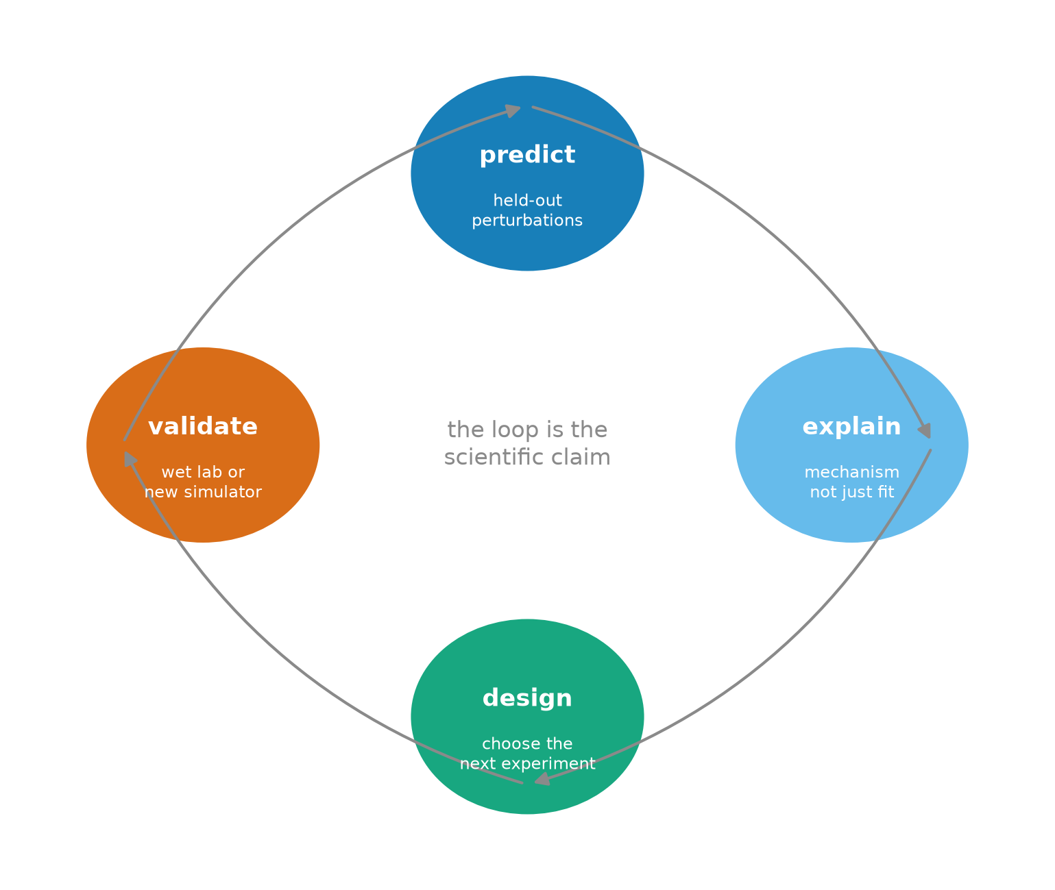
“预测—解释—设计—验证”这个闭环，是第 7 节第九条要求的操作化版本。它同时给出了评价标准：一个虚拟细胞的价值，等于它能节省的实验次数乘以那些实验的信息量。 这个量很难直接测量，但它比”在某个基准上提高了几个百分点”更接近科学的目标。

The predict–explain–design–validate loop is the operational version of requirement nine in Section 7. It also supplies the evaluation criterion: the value of a virtual cell equals the number of experiments it saves multiplied by the information those experiments would have carried. That quantity is hard to measure, but it is closer to the scientific goal than “a few points on a benchmark”.

9. 终章：当机器开始理解生命 / Coda: when a machine begins to understand life

回到开篇的问题。如果一台计算机能生成任何句子、任何图像、任何物理世界，它能不能创造生命？现在我们可以把这个问题拆成三个不同的问题，它们常常被混为一谈。

Back to the opening question. If a computer can generate any sentence, any image and any physical world, can it create life? We can now split this into three questions that are routinely conflated.

模拟（simulate） 是让一个系统的状态按规则演化，并且演化结果与某个参照一致。第 2 到第 5 节都在做这件事，而且部分做到了：语言模型模拟了语法，VAE 模拟了图像分布，两个物理模型模拟了轨迹，虚拟细胞模拟了吸引子与扰动响应。

To simulate is to let a system’s state evolve by rules such that the evolution matches some reference. Sections 2 to 5 all do this, and partly succeed: the language model simulates the grammar, the VAE simulates the image distribution, the two physical models simulate trajectories, and the virtual cell simulates attractors and perturbation responses.

理解（understand） 是另一回事。理解要求模型能回答”如果……会怎样”——包括那些从未发生、也从未被记录过的”如果”。第 5 节的图网络之所以在双敲除上远好于 MLP，正是因为它把”基因之间如何互相作用”写进了结构；而它在 200 步之后输给 MLP，又提醒我们：理解的一部分是记住世界的典型状态，而不只是写出方程。

To understand is different. Understanding requires answering “what if” — including ifs that never happened and were never recorded. The graph network in Section 5 beats the MLP on double knockouts precisely because it writes “how genes act on each other” into its structure; and the fact that it loses to the MLP after 200 steps reminds us that part of understanding is remembering the world’s typical states, not only writing equations.

创造（create） 是最强的要求：不仅是预测一个系统，而是让一个系统存在，并且它能自我维持、复制、变异、被选择。本文没有做这件事，也没有声称做了。第 5.4 节列出了三道没有跨过的门槛：进化、代谢、空间。这三道门槛中的任何一个，都足以让”虚拟细胞”与”生命”之间保持一段不可忽略的距离。

To create is the strongest requirement: not to predict a system but to bring one into existence, one that maintains itself, replicates, mutates and is selected. This article did not do that, and does not claim to. Section 5.4 lists three thresholds not crossed: evolution, metabolism, space. Any one of them keeps a non-trivial distance between “virtual cell” and “life”.

那么，如果有一天，一个虚拟细胞能准确预测从未见过的干预、能解释调控机制、能提出真实实验可以验证的假设——我们是否可以说它开始理解生命了？

So: if one day a virtual cell predicts never-seen interventions accurately, explains regulatory mechanisms, and proposes hypotheses that real experiments can verify — may we say it has begun to understand life?

我的回答是：可以，但”理解”的主体需要说清楚。 那个系统理解的是我们喂给它的那个世界——我们选择的变量、我们测量的尺度、我们允许的干预。它与真实生命之间隔着一层建模选择，而那层选择是人做的。第 6 节说过，宏观变量是我们选的，不是自然给的；这句话在这里达到了它的最终形态：一个虚拟细胞的理解，永远是”相对于某个粗粒化”的理解。

My answer: yes, but the subject of “understand” has to be named. What such a system understands is the world we fed it — the variables we chose, the scale we measured, the interventions we allowed. Between it and real life sits a layer of modelling choices, and those choices were made by people. Section 6 said that macroscopic variables are chosen by us, not handed down by nature; here that statement reaches its final form: a virtual cell’s understanding is always understanding relative to a coarse-graining.

这不是一个让人泄气的结论。恰恰相反，它解释了为什么生命模拟值得做：因为粗粒化是可以被改进的。 每一次我们把一个新的尺度、一种新的干预、一类新的观测放进模型，模型能理解的世界就变大一点。生命模拟的进展，不是某个模型突然”懂了生命”，而是我们与机器共同把”可理解的世界”向外推了一圈。

This is not a deflating conclusion. On the contrary, it explains why life simulation is worth doing: because coarse-grainings can be improved. Every time we put a new scale, a new intervention or a new kind of observation into the model, the world it can understand grows a little. Progress in life simulation is not a model suddenly “getting” life; it is humans and machines together pushing the boundary of the understandable world outward.

所以回到最初的三个房间。能写出任何句子的机器，造不出生命；能画出任何图像的机器，也造不出生命；能模拟整个物理世界的机器，理论上包含生命，但它必须先在正确的尺度上被”读”出来。生命不是被写进规则里的，也不是被画出来的，它是在正确的尺度上被组织出来的。 而这，正是虚拟细胞这件事真正难的地方，也是它值得被称为”圣殿”的地方。

So back to the three rooms. The machine that writes any sentence cannot make life; neither can the one that draws any image; the machine that simulates the entire physical world contains life in principle, but life has to be read out at the right scale. Life is not written into the rules and it is not drawn; it is organised at the right scale. That is what makes the virtual cell genuinely hard, and what makes it worth calling a sanctuary.

参考文献 / References

Turing, A. M. (1952). The chemical basis of morphogenesis. Philosophical Transactions of the Royal Society B 237, 37–72. doi:10.1098/rstb.1952.0012
Schrödinger, E. (1944). What Is Life? Cambridge University Press. (book; no DOI)
von Neumann, J. (1966). Theory of Self-Reproducing Automata (ed. A. W. Burks). University of Illinois Press. (book; no DOI)
Bedau, M. A. (1997). Weak emergence. Noûs 31, 375–399. doi:10.1111/0029-4624.31.s11.17
Hoel, E. P., Albantakis, L., & Tononi, G. (2013). Quantifying causal emergence shows that macro can beat micro. PNAS 110, 19790–19795. doi:10.1073/pnas.1314922110
Vaswani, A., et al. (2017). Attention is all you need. NeurIPS. arXiv:1706.03762
Kingma, D. P., & Welling, M. (2014). Auto-encoding variational Bayes. ICLR. arXiv:1312.6114
Ho, J., Jain, A., & Abbeel, P. (2020). Denoising diffusion probabilistic models. NeurIPS. arXiv:2006.11239
Ha, D., & Schmidhuber, J. (2018). Recurrent world models facilitate policy evolution. NeurIPS. arXiv:1809.01999
Chen, R. T. Q., Rubanova, Y., Bettencourt, J., & Duvenaud, D. (2018). Neural ordinary differential equations. NeurIPS. arXiv:1806.07366
Raissi, M., Perdikaris, P., & Karniadakis, G. E. (2019). Physics-informed neural networks. Journal of Computational Physics 378, 686–707. doi:10.1016/j.jcp.2018.10.045
Jumper, J., et al. (2021). Highly accurate protein structure prediction with AlphaFold. Nature 596, 583–589. doi:10.1038/s41586-021-03819-2
Abramson, J., et al. (2024). Accurate structure prediction of biomolecular interactions with AlphaFold 3. Nature 630, 493–500. doi:10.1038/s41586-024-07487-w
Theodoris, C. V., et al. (2023). Transfer learning enables predictions in network biology (Geneformer). Nature 618, 616–624. doi:10.1038/s41586-023-06139-9
Cui, H., et al. (2024). scGPT: toward building a foundation model for single-cell multi-omics using generative AI. Nature Methods 21, 1470–1480. doi:10.1038/s41592-024-02201-0
Roohani, Y., Huang, K., & Leskovec, J. (2024). Predicting transcriptional outcomes of novel multigene perturbations with GEARS. Nature Biotechnology 42, 927–936. doi:10.1038/s41587-023-01905-6
Bunne, C., et al. (2023). Learning single-cell perturbation responses using neural optimal transport. Nature Methods 20, 1759–1768. doi:10.1038/s41592-023-01969-x
Lotfollahi, M., et al. (2023). Predicting cellular responses to complex perturbations in high-throughput screens (CPA). Molecular Systems Biology 19, e11517. doi:10.15252/msb.202211517
Wei, J., et al. (2022). Emergent abilities of large language models. arXiv:2206.07682
Schaeffer, R., Miranda, B., & Koyejo, S. (2023). Are emergent abilities of large language models a mirage? NeurIPS. arXiv:2304.15004
Google DeepMind (2025). AlphaGenome: AI for better understanding the genome. https://deepmind.google/blog/alphagenome-ai-for-better-understanding-the-genome/
Arc Institute (2025). Virtual Cell Challenge 2025. https://virtualcellchallenge.org/2025
Arc Institute (2025). Virtual Cell Atlas. https://arcinstitute.org/tools/virtualcellatlas

说明：第 1–20 条给出 DOI 或 arXiv 编号；第 21–23 条为机构发布，给官方链接。AlphaGenome 与 Virtual Cell Challenge 的具体发布日期与赛事细节以机构页面为准。

Note: entries 1–20 carry DOIs or arXiv identifiers; 21–23 are institutional releases with official links. Dates and competition details for AlphaGenome and the Virtual Cell Challenge should be checked against those pages.